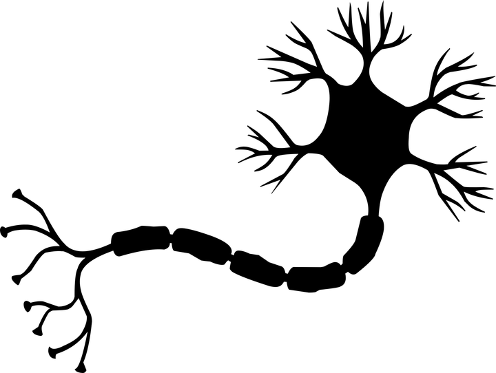
A nano-neuron is a simplified version of a neuron from the concept of a neural network. Nano-neuron performs the simplest task and is trained to convert temperature from degrees Celsius to degrees Fahrenheit.
The NanoNeuron.js code consists of 7 simple JavaScript functions involving learning, training, predicting, and direct and backward propagation of the model signal. The purpose of writing these functions was to give the reader a minimal, basic explanation (intuition) of how, after all, a machine can “learn”. The code does not use third-party libraries. As the saying goes, only simple "vanilla" JavaScript functions.
These functions are by no means an exhaustive guide to machine learning. Many machine learning concepts are missing or simplified! This simplification is allowed for the sole purpose - to give the reader the most basic understanding and intuition about how a machine can “learn” in principle, so that as a result, “MAGIC of machine learning” sounds more and more to the reader as “MATHEMATICS of machine learning”.
What our nano-neuron will “learn”
You may have heard of neurons in the context of neural networks . A nano-neuron is a simplified version of that same neuron. In this example, we will write its implementation from scratch. For simplicity, we will not build a network of nano-neurons. We will focus on creating one single nano-neuron and try to teach him how to convert temperature from degrees Celsius to degrees Fahrenheit. In other words, we will teach him to predict the temperature in degrees Fahrenheit based on the temperature in degrees Celsius.
By the way, the formula for converting degrees Celsius to degrees Fahrenheit is as follows:

But at the moment, our nano-neuron knows nothing about this formula ...
Nano-neuron model
Let's start by creating a function that describes the model of our nano-neuron. This model is a simple linear relationship between x and y , which looks like this: y = w * x + b . Simply put, our nano-neuron is a child who can draw a straight line in the XY coordinate system.
Variables w and b are model parameters . A nano-neuron knows only these two parameters of a linear function. These parameters are precisely what our nano-neuron will learn during the training process.
The only thing that a nano-neuron can do at this stage is to simulate linear relationships. He does this in the predict() method, which takes a variable x at the input and predicts the variable y at the output. No magic.
function NanoNeuron(w, b) { this.w = w; this.b = b; this.predict = (x) => { return x * this.w + this.b; } }
_ (... wait ... linear regression is you, or what?) _
Convert degrees Celsius to degrees Fahrenheit
The temperature in degrees Celsius can be converted to degrees Fahrenheit according to the formula: f = 1.8 * c + 32 , where c is the temperature in degrees Celsius and f is the temperature in degrees Fahrenheit.
function celsiusToFahrenheit(c) { const w = 1.8; const b = 32; const f = c * w + b; return f; };
As a result, we want our nano-neuron to be able to simulate this particular function. He will have to guess (learn) that the parameter w = 1.8 and b = 32 without knowing it in advance.
This is how the conversion function looks on the chart. That is what our nano-neural “baby” must learn to “draw”:

Data generation
In classical programming, we know the input data ( x ) and the algorithm for converting this data (parameters w and b ), but the output data ( y ) is unknown. The output is calculated based on the input using a known algorithm. In machine learning, on the contrary, only the input and output data ( x and y ) are known, but the algorithm for switching from x to y unknown (parameters w and b ).
It is the generation of input and output that we are now going to do. We need to generate data for training our model and data for testing the model. The celsiusToFahrenheit() helper function will help us with this. Each of the training and test data sets is a set of pairs x and y . For example, if x = 2 , then y = 35,6 and so on.
In the real world, most of the data is likely to be collected , not generated . For example, such collected data may be a set of pairs of “face photos” -> “person’s name”.
We will use the TRAINING dataset to train our nano-neuron. Before he grows up and is able to make decisions on his own, we must teach him what is “true” and what is “false” using “correct” data from a training set.
By the way, here the life principle “garbage at the entrance - garbage at the exit” is clearly traced. If a nano-neuron throws a “lie” into the training kit that 5 ° C is converted to 1000 ° F, then after many iterations of training, he will believe this and will correctly convert all temperature values except 5 ° C. We need to be very careful with the training data that we load every day into our brain neural network.
Distracted. Let's continue.
We will use the TEST dataset to evaluate how well our nano-neuron has trained and can make correct predictions on new data that he did not see during his training.
function generateDataSets() {
Prediction error estimation
We need a certain metric (measurement, number, rating) that will show how close the prediction of a nano-neuron is to true. In other words, this number / metric / function should show how right or wrong the nano neuron is. It's like in school, a student can get a grade of 5 or 2 for his control.
In the case of a nano-neuron, its error (error) between the true value of y and the predicted value of prediction will be produced by the formula:

As can be seen from the formula, we will consider the error as a simple difference between the two values. The closer the values are to each other, the smaller the difference. We use squaring here to get rid of the sign, so that in the end (1 - 2) ^ 2 equivalent to (2 - 1) ^ 2 . Division by 2 occurs solely in order to simplify the meaning of the derivative of this function in the formula for back propagation of a signal (more on this below).
The error function in this case will look like this:
function predictionCost(y, prediction) { return (y - prediction) ** 2 / 2;
Direct signal propagation
Direct signal propagation through our model means making predictions for all pairs from the xTrain and yTrain training dataset and calculating the average error (error) of these predictions.
We just let our nano-neuron “speak out”, allowing it to make predictions (convert temperature). At the same time, a nano-neuron at this stage can be very wrong. The average value of the prediction error will show us how far our model is / is close to the truth at the moment. The error value is very important here, since by changing the parameters w and b and direct signal propagation again, we can evaluate whether our nano-neuron has become “smarter” with new parameters or not.
The average prediction error of a nano-neuron will be performed using the following formula:

Where m is the number of training copies (in our case, we have 100 data pairs).
Here's how we can implement this in code:
function forwardPropagation(model, xTrain, yTrain) { const m = xTrain.length; const predictions = []; let cost = 0; for (let i = 0; i < m; i += 1) { const prediction = nanoNeuron.predict(xTrain[i]); cost += predictionCost(yTrain[i], prediction); predictions.push(prediction); }
Signal Reverse Propagation
Now that we know how our nano-neuron is right or wrong in its predictions (based on the average value of the error), how can we make the predictions more accurate?
Reverse signal propagation will help us with this. Signal back propagation is the process of evaluating the error of a nano-neuron and then adjusting its parameters w and b so that the next predictions of the nano-neuron for the entire set of training data become a little more accurate.
This is where machine learning becomes like magic. The key concept here is a derivative of the function , which shows what size step and which way we need to take in order to approach the minimum of the function (in our case, the minimum of the error function).
The ultimate goal of training a nano-neuron is to find the minimum of the error function (see function above). If we can find such values of w and b at which the average value of the error function is small, then this will mean that our nano-neuron copes well with temperature predictions in degrees Fahrenheit.
Derivatives are a large and separate topic that we will not cover in this article. MathIsFun is a great resource that can provide a basic understanding of derivatives.
One thing that we must learn from the essence of a derivative and which will help us understand how the back propagation of a signal works is that the derivative of a function at a specific point x and y , by definition, is a tangent line to the curve of this function at x and y and indicates us the direction to the minimum of the function .

Image taken from MathIsFun
For example, in the graph above, you see that at the point (x=2, y=4) slope of the tangent shows us that we need to move
The derivatives of our average error function averageCost with averageCost to the parameters w and b will look like this:


Where m is the number of training copies (in our case, we have 100 data pairs).
You can read in more detail about how to take the derivative of complex functions here .
function backwardPropagation(predictions, xTrain, yTrain) { const m = xTrain.length;
Model training
Now we know how to estimate the error / error of the predictions of our nano-neuron model for all training data (direct signal propagation). We also know how to adjust the parameters w and b the nano-neuron model (back propagation of the signal) in order to improve the accuracy of the predictions. The problem is that if we perform forward and backward propagation of the signal only once, then this will not be enough for our model to identify and learn the dependencies and laws in the training data. You can compare this to a student's one-day school visit. He / she must go to school regularly, day after day, year after year, in order to learn all the material.
So, we must repeat the forward and backward propagation of the signal many times. This is trainModel() function trainModel() . She’s like a “teacher” for the model of our nano-neuron:
- she will spend some time (
epochs ) with our still silly nano-neuron, trying to train him, - she will use special books (
xTrain and yTrain datasets) for training, - it encourages our “student” to study more diligently (faster) using the
alpha parameter, which essentially controls the speed of learning.
A few words about the alpha parameter. This is just a coefficient (multiplier) for the values of the variables dW and dB , which we calculate during the back propagation of the signal. So, the derivative showed us the direction to the minimum of the error function (the signs of the values of dW and dB tell us this). The derivative also showed us how quickly we need to move towards the minimum of the function (the absolute values of dW and dB tell us this). Now we need to multiply the step size by alpha in order to adjust the speed of our approach to a minimum (the total step size). Sometimes, if we use large values for alpha , we can go in such large steps that we can simply step over the minimum of the function, thereby skipping it.
By analogy with the “teacher”, the stronger she would force our “nano-student” to learn, the faster he would learn, BUT, if you force and put pressure on him very hard, then our “nano-student” may experience a nervous breakdown and complete apathy and he won’t learn anything at all.
We will update the parameters of our model w and b as follows:


And this is how the training itself looks:
function trainModel({model, epochs, alpha, xTrain, yTrain}) {
Putting all the features together
Time to use all previously created functions together.
Create an instance of the nano-neuron model. At the moment, the nano-neuron does not know anything about what the parameters w and b should be. So let's set w and b randomly.
const w = Math.random();
We generate training and test data sets.
const [xTrain, yTrain, xTest, yTest] = generateDataSets();
Now let's try to train our model using small steps ( 0.0005 ) for 70000 eras. You can experiment with these parameters, they are determined empirically.
const epochs = 70000; const alpha = 0.0005; const trainingCostHistory = trainModel({model: nanoNeuron, epochs, alpha, xTrain, yTrain});
Let's check how the error value of our model changed during training. We expect that the error value after training should be significantly less than before training. This would mean that our nano-neuron wiser. The opposite option is also possible, when after training, the error of predictions only increased (for example, large values of the learning step alpha ).
console.log(' :', trainingCostHistory[0]);
And here is how the value of the model error changed during training. On the x axis are epochs (in thousands). We expect that the chart will be decreasing.

Let's look at what parameters our nano-neuron “learned”. We expect that the parameters w and b will be similar to the parameters of the same name from the celsiusToFahrenheit() function ( w = 1.8 and b = 32 ), because it was her nano-neuron that I tried to simulate.
console.log(' -:', {w: nanoNeuron.w, b: nanoNeuron.b});
As you can see, the nano-neuron is very close to the celsiusToFahrenheit() function.
Now let's see how accurate the predictions of our nano-neuron are for test data that he did not see during training. The prediction error for the test data should be close to the prediction error for the training data. This will mean that the nano-neuron has learned the correct dependencies and can correctly abstract its experience from previously unknown data (this is the whole value of the model).
[testPredictions, testCost] = forwardPropagation(nanoNeuron, xTest, yTest); console.log(' :', testCost);
Now, since our "nano-baby" was well trained in the "school" and now knows how to accurately convert degrees Celsius to degrees Fahrenheit even for data that he did not see, we can call him reasonably smart. Now we can even ask him for advice on temperature conversion, and that was the purpose of the whole training.
const tempInCelsius = 70; const customPrediction = nanoNeuron.predict(tempInCelsius); console.log(`- "", ${tempInCelsius}°C :`, customPrediction);
Very close! Like people, our nano-neuron is good, but not perfect :)
Successful coding!
How to run and test a nano-neuron
You can clone the repository and run the nano neuron locally:
git clone https://github.com/trekhleb/nano-neuron.git cd nano-neuron
node ./NanoNeuron.js
Missed concepts
The following machine learning concepts have been omitted or simplified for ease of explanation.
Separation of training and test data sets
Usually you have one big data set. Depending on the number of copies in this set, its division into training and test sets can be carried out in the proportion of 70/30. The data in the set must be randomly mixed before being split. If the amount of data is large (for example, millions), then the division into test and training sets can be carried out in proportions close to 90/10 or 95/5.
Online power
Usually you will not find cases when only one neuron is used. Strength is in the network of such neurons. A neural network can learn much more complex dependencies.
Also in the example above, our nano-neuron may look more like a simple linear regression than a neural network.
Input Normalization
Before training, it is customary to normalize the input data .
Vector implementation
For neural networks, vector (matrix) calculations are much faster than calculations in for loops. Usually the direct and reverse signal propagation is performed using matrix operations using, for example, the Python Numpy library.
Minimum Error Function
The error function that we used for the nano neuron is very simplified. It should contain logarithmic components . A change in the formula for the error function will also entail a change in the formulas for the forward and backward propagation of the signal.
Activation function
Usually the output value of the neuron passes through the activation function. For activation, functions such as Sigmoid , ReLU and others can be used.