In almost any modern computer game, the presence of a physical engine is a prerequisite. Flags and rabbits fluttering in the wind, bombarded by balls - all this requires proper execution. And, of course, even if not all heroes wear raincoats ... but those who wear really need an adequate simulation of fluttering fabric.
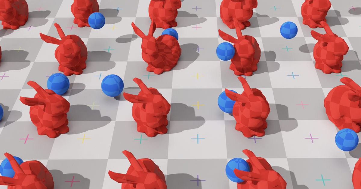
Nevertheless, full physical modeling of such interactions often becomes impossible, since it is orders of magnitude slower than necessary for real-time games. This article offers a new modeling method that can speed up physical simulations, make them 300-5000 times faster. Its purpose is to try to teach a neural network to simulate physical forces.
Progress in the development of physical engines is determined by both the growing computing power of technical equipment and the development of fast and stable modeling methods. Such methods include, for example, modeling by cutting space into subspaces and data-driven approaches - that is, based on data. The former work only in a reduced or compressed subspace, where only a few forms of deformation are taken into account. For large projects, this can lead to a significant increase in technical requirements. Data-driven approaches use the system’s memory and the pre-computed data stored in it, which reduces these requirements.
Here we look at an approach that combines both methods: in this way, it is intended to capitalize on the strengths of both. Such a method can be interpreted in two ways: either as a subspace modeling method parameterized by a neural network, or as a DD method based on subspace modeling to construct a compressed simulated medium.
Its essence is this: first we collect high-precision simulation data using
Maya nCloth , and then we calculate the linear subspace using
the principal component method (PCA) . In the next step, we use machine learning based on the classical neural network model and our new methodology, after which we introduce the trained model into an interactive algorithm with several optimizations, such as an efficient decompression algorithm by a GPU and a method for approximating vertex normals.
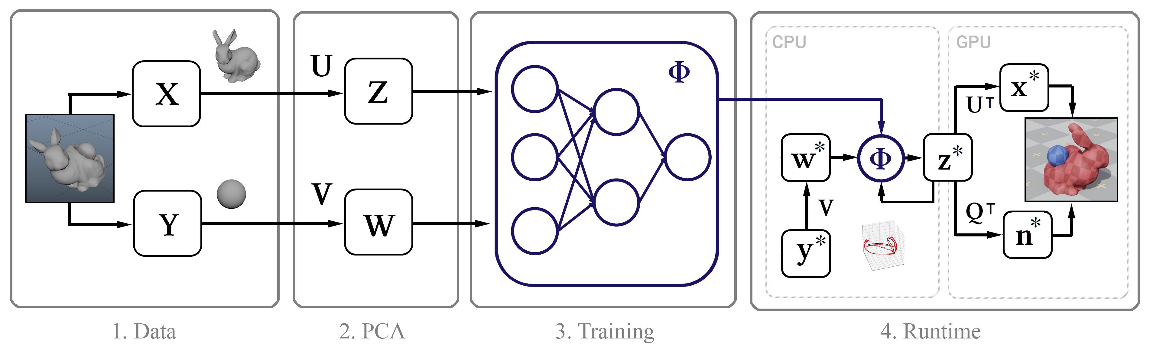 Figure 1. The structural diagram of the method
Training data
Generally speaking, the only input for this method is the raw time stamps of the frame-by-frame positions of the vertices of the object. Next, we describe the process of collecting such data.
We perform the simulation in Maya nCloth, capturing data at a speed of 60 frames per second, with 5 or 20 substeps and 10 or 25 limiting iterations, depending on the stability of the simulation. For fabrics, take a T-shirt model with a slight increase in the weight of the material and its resistance to stretching, and for deformable objects, hard rubber with reduced friction. We perform external collisions by colliding triangles of external geometry, self-collisions — vertices with vertices for fabric and triangles with triangles for rubber. In all cases, we use a rather large collision thickness - of the order of 5 cm - to ensure the stability of the model and to prevent pinching and tearing of the fabric.
Table 1. Parameters of the modeled objects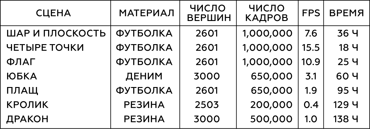
For various types of interaction of simple objects (for example, spheres), we will generate their movement in a random way by cropping random coordinates at random times. To simulate the interaction of tissue with a character, we use a motion capture database of 6.5 × 10
5 frames, which are one large animation. Upon completion of the simulation, we verify the result and exclude frames with unstable or poor behavior. For the scene with the skirt, we remove the character’s hands, since they often intersect with the geometry of the mesh of the legs and are now insignificant.
 Figure 2. The very first two scenes from the table
Usually we need 10
5 -10
6 frames of training data. In our experience, in most cases 10
5 frames is enough for testing, while the best results are achieved with 10
6 frames.
Training
Next, we will talk about the process of machine learning: about parameterization in our neural network, about network architecture and directly about the technique itself.
Parameterization
In order to obtain a training data set, we collect the coordinates of the vertices in each frame
t into one vector
x t , and then combine these frame-by-frame vectors into one large matrix X. This matrix describes the states of the modeled object. In addition, we must have an idea of the state of external objects in each frame. For simple objects (such as balls), you can use their three-dimensional coordinates, while the state of complex models (character) is described by the position of each joint relative to the reference point: in the case of a skirt, such a support will be the hip joint, in the case of a cloak - the neck. For objects with a moving reference system, the position of the Earth relative to it should be taken into account: then our system will know the direction of gravity, as well as its linear speed, acceleration, rotation speed and acceleration of rotation. For the flag, we will take into account the speed and direction of the wind. As a result, for each object we get one large vector that describes the state of the external object, and all these vectors are also combined into the matrix Y.
Now we apply the PCA to both the matrix X and Y, and use the resulting transformation matrices Z and W to construct the subspace image. If the PCA procedure requires too much memory, first sample our data.
PCA compression inevitably results in a loss of detail, especially for objects with many potential conditions, such as thin folds of fabric. However, if the subspace consists of 256 base vectors, this usually helps to preserve most of the details. Below are animations of the standard physics of the cloak and models with 256, 128 and 64 base vectors, respectively.
 Figure 3. Comparison of the control model (standard) with the models obtained by our method in spaces with different dimension bases
Source and Extended Model
It was necessary to develop a model that could predict the state of model vectors in future frames. And since the modeled objects are usually characterized by inertia with a tendency to a certain average state of rest (after the PCA procedure the object takes such a state at zero values), a good initial model would be the expression represented by line 9 of the algorithm in Figure 4. Here α and β are the model parameters, ⊙ is an exploded product. The values of these parameters will be obtained from the source data by solving the
linear least squares equation individually for α and β:

Here † is the
pseudoinverse transformation of the matrix .
Since such a prediction is only a very rough approximation and does not take into account the influence of external objects w, obviously, it will not be able to accurately model the training data. Therefore, we train the neural network Φ of approximating the residual effects of the model in accordance with the 11th line of the algorithm. Here we parameterize a standard
direct distribution neural network with 10 layers, for each layer (except the output) using the activation function
ReLU . Excluding the input and output layers, we set the number of hidden units on each remaining layer equal to one and a half the size of the PCA data, which led to a good compromise between the occupied space on the hard drive and performance.
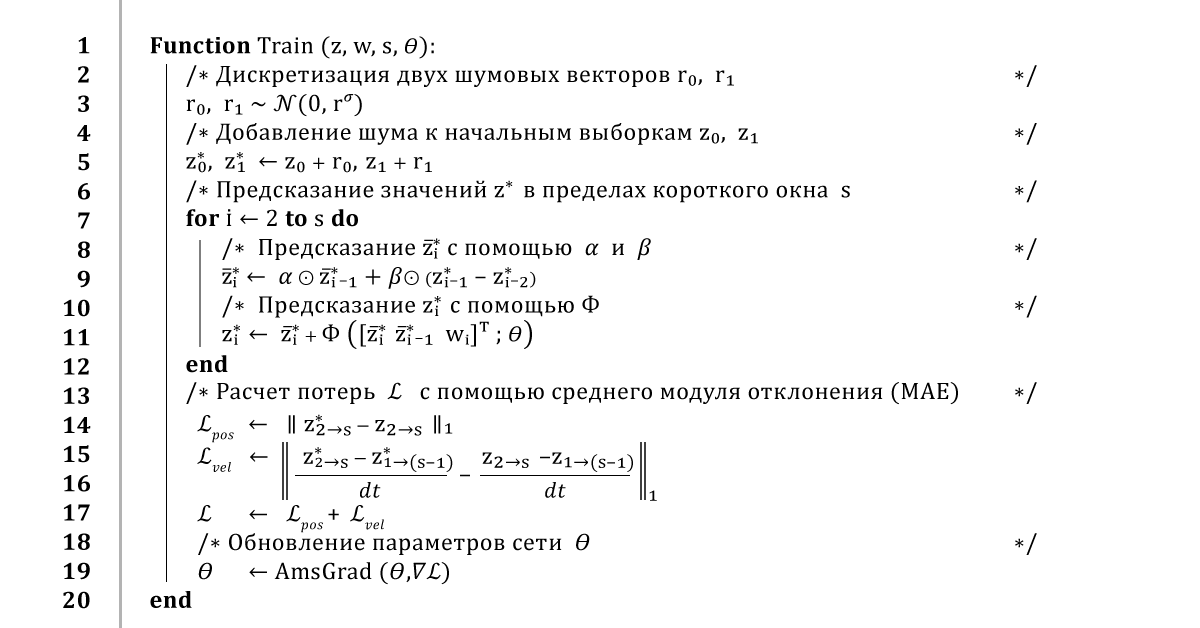 Figure 4. Neural network learning algorithm
Neural network training
A standard way to train a neural network would be to iterate over the entire data set and train the network to make predictions for each frame. Of course, such an approach will lead to a low learning error, but the feedback in such a prediction will cause unstable behavior of its result. Therefore, to ensure stable long-term prediction, our algorithm uses the
method of back propagation of errors throughout the integration procedure.
In general, it works like this: from a small window of training data
z and
w, we take the first two frames
z 0 and
z 1 and add a little noise
r 0 ,
r 1 to them , in order to slightly disrupt the learning path. Then, to predict the next frames, we run the algorithm several times, returning to the previous results of the predictions at each new time step. As soon as we get a prediction of the entire trajectory, we calculate the average coordinate error, and then pass it to the AmsGrad optimizer using the automatic derivatives calculated using TensorFlow.
We will repeat this algorithm on mini-samples of 16 frames, using overlapping windows of 32 frames, for 100 eras or until the training converges. We use the learning rate of 0.0001, the attenuation coefficient of the learning rate of 0.999, and the standard deviation of noise calculated from the first three components of the PCA space. Such training takes from 10 to 48 hours, depending on the complexity of the installation and the size of the PCA data.
 Figure 5. Visual comparison of the reference skirt and the one that our neural network learned to build
System implementation
We will describe in detail the implementation of our method in an interactive environment, including evaluating a neural network, calculating the normals to the surfaces of objects for rendering, and how we deal with visible intersections.
Rendering app
We render the resulting models in a simple interactive 3D application written in C ++ and DirectX: we once again implement the preprocesses and neural network operations in single-threaded C ++ code and load the binary network weights obtained during our training procedure. Then we apply some simple optimizations for network estimation, in particular, reuse of memory buffers and sparse vector-matrix data, which becomes possible due to the presence of zero hidden units obtained thanks to the ReLU activation function.
GPU decompression
Send compressed z state data to the GPU and decompress it for further rendering. To this end, we use a simple computational shader, which for each vertex of the object calculates the point product of the vector z and the first three rows of the matrix U
T corresponding to the coordinates of this vertex, after which we add the average value
x µ . This approach has two advantages over the
naive decompression
method . Firstly, the parallelism of the GPU significantly speeds up the calculation of the model state vector, which can take up to 1 ms. Secondly, it reduces the data transfer time between the central and the GPU by an order of magnitude, which is especially important for platforms on which the transfer of the entire state of the entire object is too slow.
Vertex Normal Prediction
During rendering, it is not enough to have access only to the coordinates of the vertices - information on the deformations of their normals is also needed. Usually, in a physical engine, either omit this calculation, or perform a naive frame-by-frame recalculation of normals with their subsequent redistribution to neighboring vertices. This may turn out to be inefficient, because the basic implementation of the central processor, in addition to the costs of decompression and data transfer, requires another 150 μs for such a procedure. And although this calculation can be performed on the GPU, it turns out to be more difficult to implement due to the need for parallel operations.
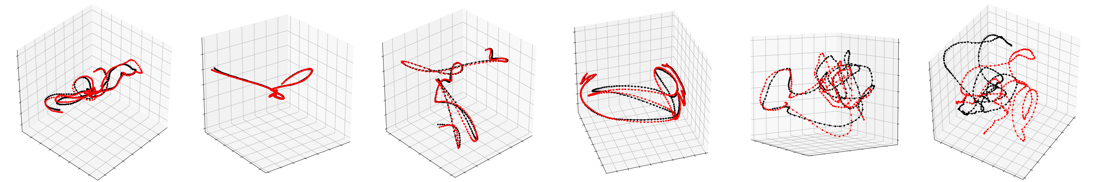
Instead, we perform a linear regression of the state of the subspace to normal full-state vectors on the GPU shader. Knowing the values of the normals of the vertices in each frame, we calculate the matrix Q, which best represents the representation of the subspace on the normals of the vertices.
Since the prediction of normals in our method has never been featured before, there is no guarantee that this approach will be accurate, but in practice it proved to be really good, as can be seen from the figure below.
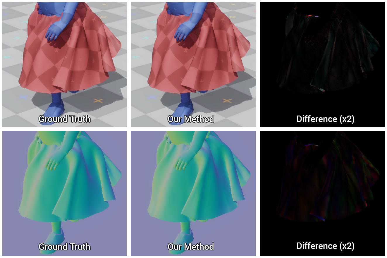 Figure 6. Comparison of the models calculated by our method and the reference (ground truth), as well as the difference between them
Intersection Fight
Our neural network learns to efficiently perform collisions, however, due to inaccuracies in predictions and errors caused by compression of the subspace, intersections may occur between external objects and simulated ones. Moreover, since we postpone the calculation of the full state of the scene until the very start of rendering, there is no way to effectively resolve these problems in advance. Therefore, to maintain high performance, eliminating these intersections is necessary during rendering.
We found a simple and effective solution for this, consisting in the fact that intersecting vertices are projected onto the surface of the primitives from which we make up the character. This projection is easy to do on the GPU using the same computational shader that decompresses the fabric and calculates the normal shading.
So, first of all, we will compose the character from the proxy objects connected with the vertices with different initial and final radii, after which we will transfer information about the coordinates and radii of these objects to the computational shader. Once again, check the coordinates of each vertex for intersection with the corresponding proxy object and, if it is, project this vertex onto the surface of the proxy object. So we only correct the position of the vertex, without touching the normal itself, so as not to damage the shading.
This approach will remove small visible intersections of objects, provided that the errors of the vertex displacement are not so large that the projection is on the opposite side of the corresponding proxy object.
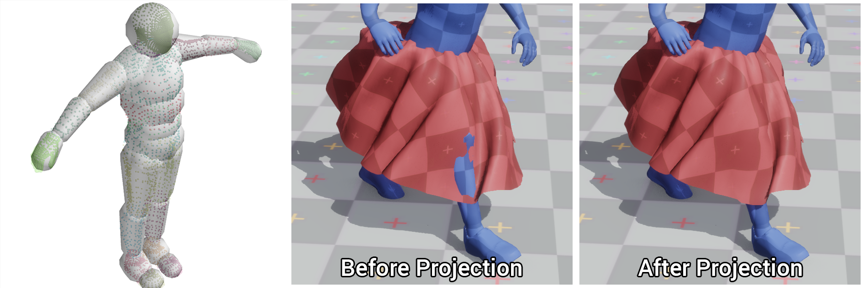 Figure 7. Character model composed of proxy objects and the results of eliminating visible intersections using our method: before and after
Results Analysis
So, our test scenes include:
, .
- 16 , 120 240 .
 8. 16 . Party time!
, , , , .
, PCA. , , , .
 9. , , –
Execution
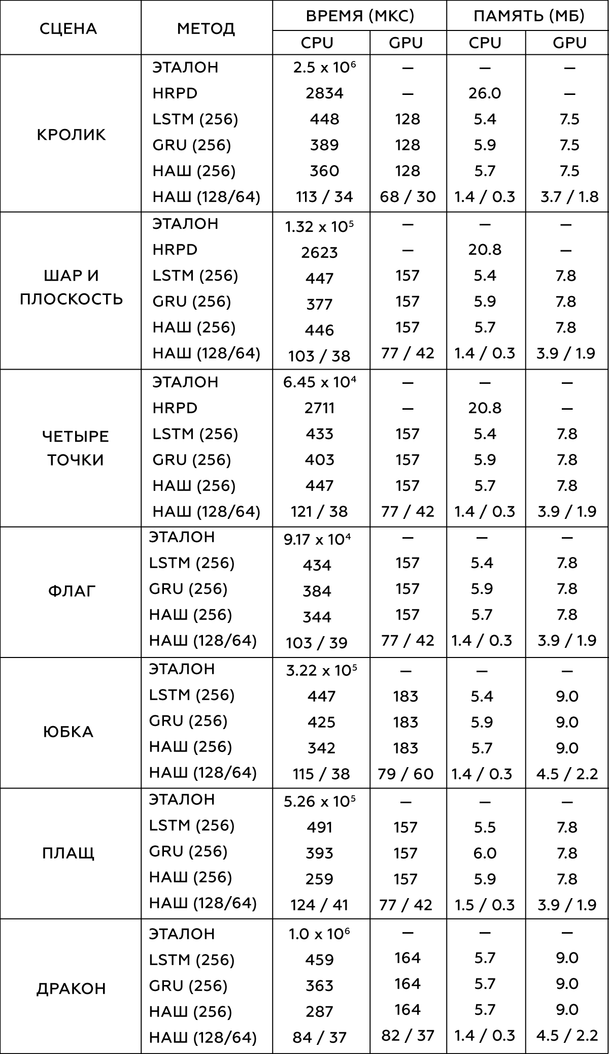
― , . , . 300-5000 , . ,
- (HRPD) ,
(LSTM) (GRU) .
, . Intel Xeon E5-1650 3.5 GHz GeForce GTX 1080 Titan.
2.
, , . , .
data-driven , . , , , , , . , , ― , .
, , , .
, . data-driven , ― , . , , , . , , , .
, . .
, , , . , , ― , . -, , , - . .
, , , , . , , , , ― , , . .
.
 10. vs : choose your fighter