大型或小型公司一位非常真实的首席分析师的任务是“研究分析师空缺市场”。 解析器使用hh手动打包数十个工作描述,根据要求的技能将其分散,并在相应的电子表格列中增加计数器。
我在这项任务中看到了一个自动化的好领域,因此决定尝试以更少的血液来轻松,简单地应对它。
我对本研究中提出的以下问题感兴趣:
- 业务和系统分析师的平均工资,
- 在这个职位上最需要的技能和个人素质,
- 某些技能和薪水水平之间的依赖关系(如果有)。
剧透:它并不容易,简单地解决。
资料准备
如果我们要收集有关职位空缺的大量数据,那么逻辑上是不受限制的。 但是,对于 实验纯度 简单起见,我们从此资源开始。
收藏品
为了收集数据,我们将通过hh API使用职位搜索 。
我将使用简单的文本查询“系统分析师”,“业务分析师”和“产品负责人”进行搜索,因为通常这些职位的活动和职责范围重叠。
为此,创建一个格式为https://api.hh.ru/vacancies?text="systems+analyst"的请求,然后解析接收到的JSON。
为了获得样本中最相关的空缺,我们将在搜索中添加search_field=name参数,仅在空缺标题中进行搜索。
在这里,您可以查看为该请求返回的空缺字段。 我选择了以下内容:
- 职称
- 城市
- 出版日期
- 薪水-上下限
- 表示工资的货币
- 总-T / F
- 公司
- 责任
- 候选人要求
此外,我想进一步分析“关键技能”部分中指示的技能,但是此部分仅在完整的职位描述中可用。 因此,我还将保留指向找到的职位的链接,以便随后获得每个职位的技能列表。
查看代码 # :) library(jsonlite) library(curl) library(dplyr) library(ggplot2) library(RColorBrewer) library(plotly) hh.getjobs <- function(query, paid = FALSE) { # Makes a call to hh API and gets the list of vacancies based on the given search queries df <- data.frame( query = character() # , URL = character() # , id = numeric() # id , Name = character() # , City = character() , Published = character() , Currency = character() , From = numeric() # . , To = numeric() # . , Gross = character() , Company = character() , Responsibility = character() , Requerement = character() , stringsAsFactors = FALSE ) for (q in query) { for (pageNum in 0:99) { try( { data <- fromJSON(paste0("https://api.hh.ru/vacancies?search_field=name&text=\"" , q , "\"&search_field=name" , "&only_with_salary=", paid ,"&page=" , pageNum)) df <- rbind(df, data.frame( q, data$items$url, as.numeric(data$items$id), data$items$name, data$items$area$name, data$items$published_at, data$items$salary$currency, data$items$salary$from, data$items$salary$to, data$items$salary$gross, data$items$employer$name, data$items$snippet$responsibility, data$items$snippet$requirement, stringsAsFactors = FALSE)) }) print(paste0("Downloading page:", pageNum + 1, "; query = \"", q, "\"")) } } names <- c("query", "URL", "id", "Name", "City", "Published", "Currency", "From", "To", "Gross", "Company", "Responsibility", "Requirement") colnames(df) <- names return(df) }
在hh.getjobs()函数中,输入接受我们感兴趣和精细化的搜索查询向量,我们仅对具有指定薪水或连续的职位空缺感兴趣(默认情况下,我们选择第二个选项)。 创建一个空的fromJSON()框架,然后jsonlite fromJSON()包的fromJSON()函数,该函数获取输入URL并返回结构化列表。 接下来,从该列表中的节点中,我们获得我们感兴趣的数据,并填写相应的数据框字段。
默认情况下,数据是逐页给出的,每页上有20个元素。 最多提供2,000个职位空缺。 我们收到的所有数据都记录在df 。
人生攻略1:完全没有应我们的要求提供2,000个空缺的事实,从某个时候开始我们将收到空白页。 在这种情况下,R发誓并跳出循环。 因此,我们小心地将内部循环的内容包装在try() 。
生活技巧2:在内部循环中将当前数据收集状态的输出添加到控制台也很有意义,因为这不是一项快速的业务。 我这样做:
print(paste0("Downloading page:", pageNum + 1, "; query = \"", query, "\""))
填写数据后,将对列进行重命名,以便于使用它们,并返回结果数据框。
我将将此功能和其他辅助功能存储在单独的functions.R文件中,以免使主脚本混乱,到目前为止,它看起来像这样:
source("functions.R") # Step 1 - get data # 1.1 get vacancies (short info) jobdf <- hh.getjobs(query = c("business+analyst" , "systems+analyst" , "product+owner"), paid = FALSE)
现在,我们将从完整的职位描述中获得experience和key_skills 。
hh.getxp将数据帧传递给hh.getxp函数,通过保存的空缺链接,并从完整的描述中获得所需工作经验的价值。 结果值存储在新列中。
查看代码 hh.getxp <- function(df) { df$experience <- NA for (myURL in df$URL) { try( { data <- fromJSON(myURL) df[df$URL == myURL, "experience"] <- data$experience$name } ) print(paste0("Filling in ", which(df$URL == myURL, arr.ind = TRUE), "from ", nrow(df))) } return(df) }
新辅助函数的描述发送到functions.R ,主脚本现在可以访问它:
# s.1.2 get experience (from full info) jobdf <- hh.getxp(jobdf) # 1.3 get skills (from full info) all.skills <- hh.getskills(jobdf$URL)
在上面的片段中,我们还形成了一个新的数据框架all.skills形式为“工作all.skills技能”:
查看代码 hh.getskills <- function(allurls) { analyst.skills <- data.frame( id = character(), # id skill = character() # ) for (myURL in allurls) { data <- fromJSON(myURL) if (length(data$key_skills) > 0) analyst.skills <- rbind(analyst.skills, cbind(data$id, data$key_skills)) print(paste0("Filling in " , which(allurls == myURL, arr.ind = TRUE) , " out of " , length(allurls))) } names(analyst.skills) <- c("id", "skill") analyst.skills$skill <- tolower(analyst.skills$skill) return(analyst.skills) }
前处理
让我们看看我们设法收集了多少数据:
> length(unique(jobdf$id)) [1] 1478 > length(jobdf$id) [1] 1498
几乎有半个工作! 看起来不错 显然,有几个空缺两次进入了搜索结果-针对不同的请求。 因此,第一步是仅保留唯一的条目: jobdf <- jobdf[unique(jobdf$id),] 。
为了比较劳动力市场分析师的薪水,我需要
1)确保所有可用薪金数据均以单一货币显示,
2)在一个单独的数据框中选择要显示工资的职位空缺。
我们将更详细地考虑每个子任务。 以前,您可以使用table(jobdf$Currency)找出原则上在我们的数据中找到table(jobdf$Currency) 。 就我而言,除了卢布之外,还出现了美元,欧元,格里夫纳汇率,哈萨克坚戈甚至乌兹别克斯坦的钱。
要将薪水值转换为卢布,您需要找出当前汇率。 我们将从中央银行了解 :
查看代码 quotations.update <- function(currencies) { # Parses the most up-to-date qutations data provided by the Central Bank of Russia # and returns a table with currency rate against RUR doc <- XML::xmlParse("http://www.cbr.ru/scripts/XML_daily.asp") quotationsdf <- XML::xmlToDataFrame(doc, stringsAsFactors = FALSE) quotationsdf <- select(quotationsdf, -Name) quotationsdf$NumCode <- as.numeric(quotationsdf$NumCode) quotationsdf$Nominal <- as.numeric(quotationsdf$Nominal) quotationsdf$Value <- as.numeric(sub(",", ".", quotationsdf$Value)) quotationsdf$Value <- quotationsdf$Value / quotationsdf$Nominal quotationsdf <- quotationsdf %>% select(CharCode, Value) return(quotationsdf) }
为了确保在R中正确处理课程,您需要确保小数点由点分隔。 此外,您应注意“名义”栏:1处为10或100处。这表示一英镑的价格约为85卢布,例如,对于一百亚美尼亚德拉姆,您可以购买〜13卢布。 为了方便进一步处理,我将这些值减小到相对于卢布的名义值1。
现在您可以翻译了。 我们的脚本使用convert.currency()函数执行此操作。 当前的汇率是从quotations表中获取的,在该表中我们从中央银行提供的XML中保存了数据。 同样,输入函数接受要转换的目标货币(默认情况下为RUR)和带有空缺的表,即需要产生单一货币的薪水分叉的值。 该函数返回具有更新的薪水数字的表格(已经没有“货币”列,这是不必要的)。
我不得不修改白俄罗斯卢布:在以几种方法接收到非常奇怪的数据之后,我进行了一次小型研究,发现自2016年以来白俄罗斯使用了一种新货币,这种新货币不仅汇率不同,而且缩写也不同(现在不是BYR,而是BYN)。 。 在hh 目录中 ,仍使用BYR缩写,关于中央银行的XML不知道什么。 因此,在函数convert.currency()我 不以最优雅的方式 首先,我用当前的缩写代替缩写,然后才直接进行转换。
看起来像这样:
查看代码 convert.currency <- function(targetCurrency = "RUR", df, quotationsdf) { cond <- (!is.na(df$Currency) & df$Currency == "BYR") df[cond, "Currency"] <- "BYN" currencies <- unique(na.omit(df$Currency[df$Currency != targetCurrency])) # ( ) if (!is.null(df$From)) { for (currency in currencies) { condition <- (!is.na(df$From) & df$Currency == currency) try( df$From[condition] <- df$From[condition] * quotationsdf$Value[quotationsdf$CharCode == currency] ) } } # ( ) if (!is.null(df$To)) { for (currency in currencies) { condition <- !is.na(df$To) & df$Currency == currency try( df$To[condition] <- df$To[condition] * quotationsdf$Value[quotationsdf$CharCode == currency] ) } } return(df %>% select(-Currency)) }
您还可以考虑到某些薪水数据是以总值表示的,也就是说,员工的手头薪水会少一些。 要计算俄罗斯联邦居民的净工资,必须从这些数字中扣除13%(非居民则扣除30%)。
查看代码 gross.to.net <- function(df, resident = TRUE) { if (resident == TRUE) coef <- 0.87 else coef <- 0.7 if (!is.null(df$Gross)) { if (!is.null(df$From)) # ( ) { index <- na.omit(as.numeric(rownames(df[!is.na(df$From) & df$Gross == TRUE,]))) df$From[index] <- df$From[index] * coef } if (!is.null(df$To)) # ( ) { index <- na.omit(as.numeric(rownames(df[!is.na(df$To) & df$Gross == TRUE,]))) df$To[index] <- df$To[index] * coef } df <- df %>% select(-Gross) } return(df) }
当然,我不会这样做,因为在这种情况下,有必要考虑不同国家(而不仅仅是俄罗斯)的税收,或者在初始搜索查询中按国家/地区添加过滤条件。
分析之前的最后一步是将找到的职位空缺分为三类:六月,中级和高级职位,并将收到的职位写在新列中。 高级职位将包括名称中出现单词“ senior”及其同义词的职位。 同样,我们将找到关键字“ junior”和同义词的起始位置,并且在中间位置中包括以下所有中间位置:
get.positions <- function(df) { df$lvl <- NA df[grep(pattern = "lead|senior|||", x = df$Name, ignore.case = TRUE), "lvl"] <- "senior" df[grep(pattern = "junior|||", x = df$Name, ignore.case = TRUE), "lvl"] <- "junior" df[is.na(df$lvl), "lvl"] <- "middle" return(df) }
将数据准备块添加到主脚本中。
已添加 # Step 2 - prepare data # 2.1. Convert all currencies to target currency # 2.1.1 get up-to-date currency rates quotations <- quotations.update() # 2.1.2 convert to RUR jobdf <- convert.currency(df = jobdf, quotationsdf = quotations) # 2.2 convert Gross to Net # jobdf <- gross.to.net(df = jobdf) # 2.3 define segments jobdf <- get.positions(jobdf)
分析方法
如上所述,我将分析所获得数据的以下方面:
- 平均工资BA / SA,
- 在这个职位上最需要的技能和个人素质,
- 某些技能和薪水水平之间的依赖关系(如果有)。
BA / SA平均收入
事实证明,公司不愿指出工资的上限或下限。
在我们的数据框jobdf这些值分别在“收件人”和“发件人”列中。 我想查找平均值并将其写入新的薪金列。
对于薪水全部显示的情况,可以使用mean()函数轻松完成此操作,过滤掉插头上的数据全部或部分丢失的所有其他记录。 但是在这种情况下,我们的原始样本(现在已经很小)所剩不到10%。 因此,我计算系数 Podgoniana ,它告诉您在指示完整叉的空缺中,“ To”和“ From”值平均相差多少,并且在只有一个值缺失的情况下,借助它的帮助,我可以填写缺失的数据。
查看代码 select.paid <- function(df, suggest = TRUE) { # Returns a data frame with average salaries between To and From # optionally, can suggest To or From value in case only one is specified if (suggest == TRUE) { df <- df %>% filter(!is.na(From) | !is.na(To)) magic.coefficient <- # shows the average difference between max and min salary round(mean(df$To/df$From, na.rm = TRUE), 1) df[is.na(df$To),]$To <- df[is.na(df$To),]$From * magic.coefficient df[is.na(df$From),]$From <- df[is.na(df$From),]$To / magic.coefficient } else { df <- na.omit(df) } df$salary <- rowMeans(x = df %>% select(From, To)) df$salary <- ceiling(df$salary / 10000) * 10000 return(df %>% select(-From, -To)) }
这是一个“软”数据过滤,它在select.paid()函数中使用suggest = TRUE参数进行设置。 或者,我们可以在调用函数时指定suggest = FALSE ,并简单地剪掉至少部分缺少薪水数据的所有行。 但是,使用软过滤和魔术系数,我设法将样本中原始数据集的近四分之一保存了下来。
我们转到视觉部分:

在此图上,您可以直观地评估BA / SA薪水在两个首都和地区的分布密度。 但是,如果我们指定请求并比较首都的中层和高层有多少呢?
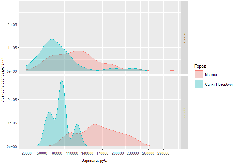
从所获得的图表中可以清楚地看出,莫斯科和圣彼得堡的中高级男性之间的薪资状况差异并没有太大差异。 因此,在圣彼得堡,中产阶级通常获得约70 tr的收入,而在莫斯科,密度峰值约为120 tr,莫斯科和圣彼得堡的高级专家的收入差异平均相差6万。
例如,我们还可以按位置查看分析师的莫斯科薪酬:

可以得出的结论是:a)今天,莫斯科对入门级分析师的需求更大; b)同时,此类专家的最高工资门槛比中级和高级员工的门槛高得多。
另一个观察结果:莫斯科中高级专家的平均相交面积相当大。 这可能表明市场在这两个步骤之间的边界相当模糊。
切割后图表的完整代码。
检视 # Step 3 - analyze salaries # 3.1 get paid jobs (with salaries specified) jobs.paid <- select.paid(jobdf) # 3.2 plot salaries density by region ggplotly(ggplot(jobs.paid, aes(salary, fill = region, colour = region)) + geom_density(alpha=.3) + scale_fill_discrete(guide = guide_legend(reverse=FALSE)) + scale_x_continuous(labels = function(x) format(x, scientific = FALSE), name = ", .", breaks = round(seq(min(jobs.paid$salary), max(jobs.paid$salary), by = 30000),1)) + scale_y_continuous(name = " ") + theme(axis.text.x = element_text(size=9), axis.title = element_text(size=10))) # 3.3 compare salaries for middle / senior in capitals ggplot(jobs.paid %>% filter(region %in% c("", "-"), lvl %in% c("senior", "middle")), aes(salary, fill = region, colour = region)) + facet_grid(lvl ~ .) + geom_density(alpha = .3) + scale_x_continuous(labels = function(x) format(x, scientific = FALSE), name = ", .", breaks = round(seq(min(jobs.paid$salary), max(jobs.paid$salary), by = 30000),1)) + scale_y_continuous(name = " ") + scale_fill_discrete(name = "") + scale_color_discrete(name = "") + guides(fill=guide_legend( keywidth=0.1, keyheight=0.1, default.unit="inch") ) + theme(legend.spacing = unit(1,"inch"), axis.title = element_text(size=10)) # 3.4 plot salaries in Moscow by position ggplotly(ggplot(jobs.paid %>% filter(region == ""), aes(salary, fill = lvl, color = lvl)) + geom_density(alpha=.4) + scale_fill_brewer(palette = "Set2") + scale_color_brewer(palette = "Set2") + theme_light() + scale_y_continuous(name = " ") + scale_x_continuous(labels = function(x) format(x, scientific = FALSE), name = ", .", breaks = round(seq(min(jobs.paid$salary), max(jobs.paid$salary), by = 30000),1)) + theme(axis.text.x = element_text(size=9), axis.title = element_text(size=10)))
关键技能分析
我们继续研究的主要目标-确定BA / SA最受欢迎的技能。 为此,我们将分析在职位空缺的特殊领域-关键技能中明确指出的数据。
最受欢迎的技能
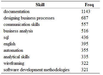
之前,我们收到了一个单独的数据帧all.skills ,在其中记录了“ job id-skill”对。 使用table()函数可以轻松找到最常见的技能:
tmp <- as.data.frame(table(all.skills$skill), col.names = c("Skill", "Freq")) htmlTable::htmlTable(x = head(tmp[order(tmp$Freq, na.last = TRUE, decreasing = TRUE),]), rnames = FALSE, header = c("Skill", "Freq"), align = 'l', css.cell = "padding-left: .5em; padding-right: 2em;")
您会得到如下内容:

Freq是“ key_skills”字段中的空缺数量,该空缺数量指示了“技能”列中的相应技能。
“但这还不是全部!”(C)很明显,在不同的空缺中可以用同义词轻松地找到相同的技能。
我为技能名称编写了一个小的同义词词典,并将其分为几类。
该词典是一个带有类别列的csv文件-以下内容之一:活动,工具,知识,标准和个人; 技能-技能的主要名称,我将使用它代替找到的所有同义词; syn1,syn2,... syn13-每个技能的实际可能变化。 某些行可能包含同义词的空列。
category;skill;syn1;syn2;syn3;syn4;syn5;syn6;syn7;syn8;syn9;syn10;syn11;syn12;syn13 tools;axure;;;;;;;;;;;;; tools;lucidchart;;;;;;;;;;;;; standards;archimate;;;;;;;;;;;;; standards;uml;activity diagram;use case diagram;ucd;class diagram;;;;;;;;; personal;teamwork;team player; ;;;;;;;;;;; activities;wireframing;mockup;mock-up;;-;wireframe;;ui;ux/;/ux;;;;
首先,导入字典,然后根据现有的等效项再次重新分配技能:
# Analyze skills # 4.1 import dictionary dict <- read.csv(file = "competencies.csv", header = TRUE, stringsAsFactors = FALSE, sep = ";", na.strings = "", encoding = "UTF-8") # 4.2 match skills with dictionary all.skills <- categorize.skills(all.skills, dict)
在剪切下,您可以看到categorize.skills()函数的填充。
那些胆量大! categorize.skills <- function(analyst_skills, dictionary) { analyst_skills$skill.group <- NA analyst_skills$category <- NA for (myskill in dictionary$skill) { category <- dictionary[dictionary$skill == myskill, "category"] mypattern <- paste0(na.omit(t(dictionary %>% filter(skill == myskill) %>% select(starts_with("syn")))), collapse = "|") if (nchar(mypattern) > 1) mypattern <- paste0(c(myskill, mypattern), collapse = "|") else mypattern <- myskill try( { analyst_skills[grep(x = analyst_skills$skill, pattern = mypattern),"skill.group"] <- myskill analyst_skills[grep(x = analyst_skills$skill, pattern = mypattern),"category"] <- category } ) } return(analyst_skills) }
我将类别和技能列添加到原始技能数据框中。 组-分别表示技能的类别和通用名称。 然后,我检查了导入的字典,并从同义词的每一行组成了grep()函数的模式。 通过将每个非空列值添加到该行,我用破折号将它们分开以获得“或”条件。 因此,对于源表中的所有技能(包括uml|activity diagram|use case diagram|ucd|class diagram ,我将在skill.group列中写入值“ uml”。 所有人的技能也是如此!..原始数据帧中的技能。
通过重新请求最流行的技能,您可以看到力量的排列有所变化:
这三位领导人现在拥有项目管理,业务分析和文档编制,而UML的知识已从前7名转移到了7名。
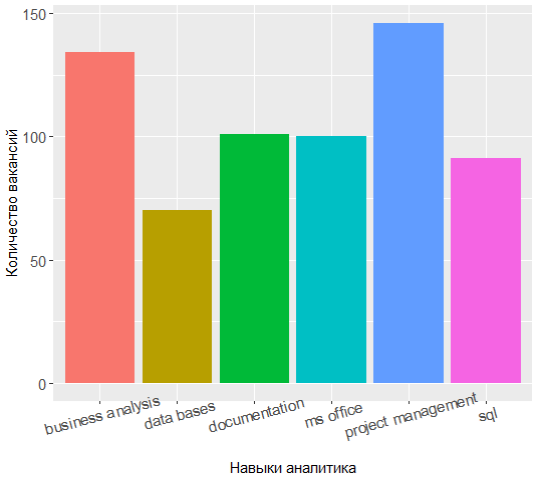
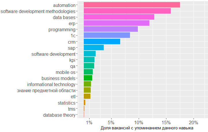
仔细研究类别并找出每种类别中最需要的技能是非常有趣的。
例如,对于知识类别,情况如下:
查看代码 tmp <- merge(x = all.skills, y = jobdf %>% select(id, lvl), by = "id", sort = FALSE) tmp <- na.omit(tmp) ggplot(as.data.frame(table(tmp %>% filter(category == "knowledge") %>% select(skill.group)))) + geom_bar(colour = "#666666", stat = "identity", aes(x = reorder(Var1, Freq), y = Freq, fill = reorder(Var1, -Freq))) + scale_y_continuous(name = " ") + theme(legend.position = "none", axis.text = element_text(size = 12)) + coord_flip()

该图显示对数据库,软件开发方法和1C领域的知识的最大需求。 接下来是CRM,ERP系统和编程基础方面的知识。
就标准而言,确实非常需要SQL和UML的知识,ARIS标记紧随其后,但GOST仅占据第六位。
这是代码 ggplot(as.data.frame(table(tmp %>% filter(category == "standards") %>% select(skill.group)))) + geom_bar(colour = "#666666", stat = "identity", aes(x = reorder(Var1, Freq), y = Freq, fill = Var1)) + scale_y_continuous(name = " ") + theme(legend.position = "none", axis.text = element_text(size = 12)) + coord_flip()

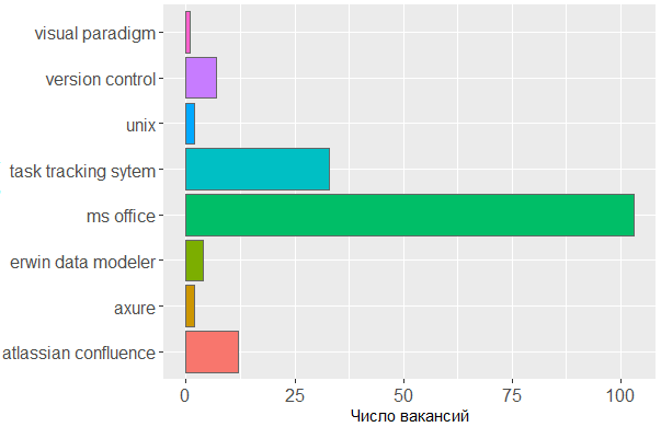
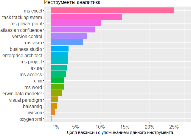
至于使用过的工具,我们再次看到确认头是分析人员的主要工具。 一个人离不开MS Office生产线和任务跟踪系统,但是剩下的部分对于编辑人员来说无关紧要,分析师可以在其中创建自己的方案或绘制界面模型。
这是代码 ggplot(tmp %>% filter(category == "tools")) + geom_histogram(colour = "#666666", stat = "count", aes(skill.group, fill = skill.group)) + scale_y_continuous(name = " ") + theme(legend.position = "none", axis.text = element_text(size = 12)) + coord_flip()
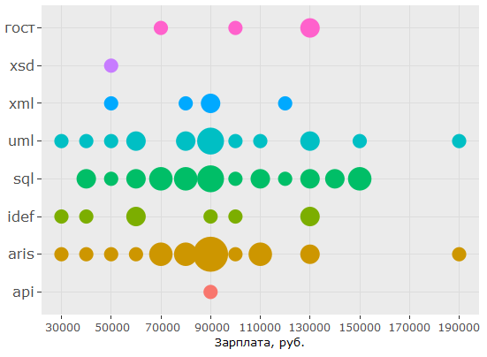
技能对收入的影响
, , . , , , .
jobs.paid all.skills , data frame.
# 4.4 vizualize paid skills tmp <- na.omit(merge(x = all.skills, y = jobs.paid %>% select(id, salary, lvl, City), by = "id", sort = FALSE))
:
> head(tmp) id skill skill.group category salary lvl City 2 25781585 android mobile os knowledge 90000 middle 3 25781585 project management activities 90000 middle 5 25781585 project management activities 90000 middle 6 25781585 ios mobile os knowledge 90000 middle 7 25750025 aris aris standards 70000 middle 8 25750025 - business analysis activities 70000 middle
, .. . :
ggplotly(ggplot(tmp %>% filter(category == "activities"), aes(skill.group, salary)) + coord_flip() + geom_count(aes(size = ..n.., color = City)) + scale_fill_discrete(name = "") + scale_y_continuous(name = ", .") + scale_size_area(max_size = 11) + theme(legend.position = "bottom", axis.title = element_blank(), axis.text.y = element_text(size=10, angle=10)))

, BA/SA .
:
ggplot(tmp %>% filter(category == "personal", City %in% c("", "-")), aes(tools::toTitleCase(skill), salary)) + coord_flip() + geom_count(aes(size = ..n.., color = skill.group)) + scale_y_continuous(breaks = round(seq(min(tmp$salary), max(tmp$salary), by = 20000),1), name = ", .") + scale_size_area(max_size = 10) + theme(legend.position = "none", axis.title = element_text(size = 11), axis.text.y = element_text(size=10, angle=0))
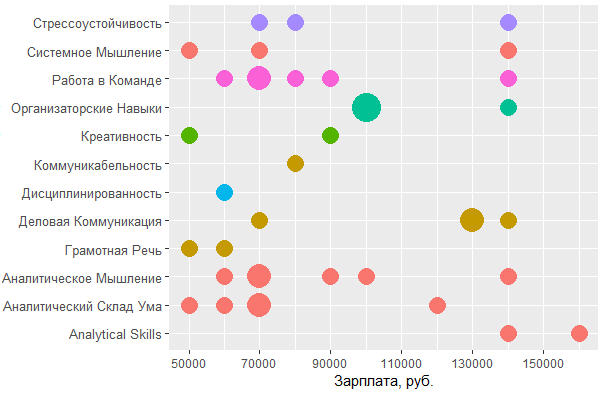
, MS Office , — , - . , , , .
, , : UML ARIS, SQL ( ) , IDEF — , "".
, , , . , 1478 - key_skills. , - .
, data frame:
> jobdf$Responsibility[[1]] [1] "Training course in business analysis. ● Define needs of the user/client, understand the problem which needs to be solved. ● " > jobdf$Requirement[[1]] [1] "At least 6 months' experience in business analysis. ● Knowledge of qualitative methods such as usability testing, interviewing, focus groups. ● "
, , . URL' , .
hh.get.full.desrtion <- function(df) { df$full.description <- NA for (myURL in df$URL) { try( { data <- fromJSON(myURL) if (length(data$description) > 0) { df$full.description[which(df$URL == myURL, arr.ind = TRUE)] <- data$description } print(paste0("Filling in " , which(df$URL == myURL, arr.ind = TRUE) , " out of " , length(df$URL))) } ) } df$full.description <- tolower(df$full.description) return(df) }
- , html- ., gsub :
remove.Html <- function(htmlString) { #remove html tags return(gsub("<.*?>", "", htmlString)) }
, , , , . data frame ( df), , df "id, skill.group, category".
skills.from.desc <- function(df, dictionary) { sk <- data.frame( id = numeric() , skill.group = character() , category = character() ) for (myskill in dictionary$skill) { category <- dictionary[dictionary$skill == myskill, "category"] mypattern <- paste0(na.omit(t(dictionary %>% filter(skill == myskill) %>% select(starts_with("syn")))), collapse = "|") if (nchar(mypattern) > 1) { mypattern <- paste0(c(myskill, mypattern), collapse = "|") } else { mypattern <- myskill } cond = grep(x = df$full.description, pattern = mypattern) tmp <- data.frame( id = df[cond, "id"], skill.group = rep(myskill, length(cond)), category = rep(category, length(cond)) ) sk <- rbind(sk, tmp) } return(sk) }
# 5 text analysis # 5.1 get full descriptions jobdf <- hh.get.full.description(jobdf) jobdf$full.description <- remove.Html(tolower(jobdf$full.description)) sk.from.desc <- skills.from.desc(jobdf, dict)
, ?
> head(sk.from.desc) id skill.group category 1 25638419 axure tools 2 24761526 axure tools 3 25634145 axure tools 4 24451152 axure tools 5 25630612 axure tools 6 24985548 axure tools > tmp <- as.data.frame(table(sk.from.desc$skill.group), col.names = c("Skill", "Freq")) > htmlTable::htmlTable(x = head(tmp[order(tmp$Freq, na.last = TRUE, decreasing = TRUE),], 20), rnames = FALSE, header = c("Skill", "Freq"), align = 'l', css.cell = "padding-left: .5em; padding-right: 2em;")
, ! Project management, key_skills, ( ).
, , key_skills -5.
, . 1478 , , key_skills, , .
, , BA , - .
, .
data frame , , . , -.
tmp <- na.omit(merge(x = sk.from.desc, y = jobs.paid %>% filter(City %in% c("", "-")) %>% select(id, salary, lvl, City), by = "id", sort = FALSE))
> head(tmp) id skill.group category salary lvl City 1 25243346 uml standards 160000 middle 2 25243346 requirements management activities 160000 middle 3 25243346 designing business processes activities 160000 middle 4 25243346 communication skills personal 160000 middle 5 25243346 mobile os knowledge 160000 middle 6 25243346 ms visio tools 160000 middle
, , , .
ggplotly(ggplot(tmp %>% filter(category == "activities"), aes(skill.group, lvl)) + geom_count(aes(color = salary, size = ..n..)) + scale_size_area(max_size = 13) + theme(legend.position = "right", legend.title = element_text(size = 10), axis.title = element_blank(), axis.text.y = element_text(size=10)) + coord_flip() + scale_color_continuous(labels = function(x) format(x, scientific = FALSE), breaks = round(seq(min(tmp$salary), max(tmp$salary), by = 70000),1), low = "blue", high = "red", name = ", ."))
?
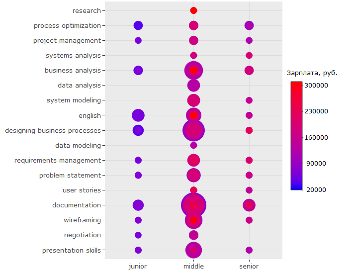
-, , - . ( , , , .)
-, , "" -, .
, key_skills.
, , 150 .. UML ARIS, IDEF, , — .
:

, - , , key_skills , . , 150 .. , .
?
, - :

, , , ? , . , , . , ó ( )
, - :

-
BA/SA ,
- . , ;
- ( ) 200 .. , , ;
- ;
- — - ( , , )
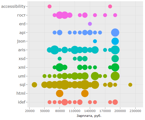
key_skills hh , ;- , , , (!) ;
- , -, UX ;
- . , - 150 ..;
- , , SQL, UML & ARIS. , .. . , , ,
wordcloud2::wordcloud2(data = table(sk.from.desc$skill.group), rotateRatio = 0.3, color = 'random-dark')
