简介:
在许多技术设备的数学建模中,使用了微分非线性方程组。 这些模型不仅用于技术中,而且还用于经济学,化学,生物学,医学和管理中。
对这种设备的功能的研究需要解决这些方程组。 由于此类方程的大部分是非线性且非平稳的,因此通常无法获得其解析解。
需要使用数值方法,其中最著名的是Runge – Kutta方法[1]。 至于Python,在数值方法的出版物中,例如[2,3],关于使用Runge – Kutta的数据很少,也没有关于对Runge – Kutta – Felberg方法进行修改的数据。
当前,由于其简单的界面,scipy.integrate模块中的odeint函数在Python中的分布最大。 该模块的第二个功能ode实现了多种方法,包括上述提到的五级Runge-Kutta-Felberg方法,但是由于其通用性,其性能有限。
本出版物的目的是对列出的方法进行比较分析,该方法用于使用Runge-Kutta-Felberg方法在Python下用修改的作者对微分方程组进行数值求解。 该出版物还提供了针对微分方程(SDE)系统的边值问题的解决方案。
有关CDS数值解算方法和软件的简要理论和实际数据
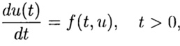
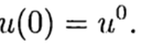
柯西的问题对于一个n阶微分方程,柯西问题在于找到一个满足等式的函数:
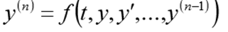
和初始条件

在解决此问题之前,应以以下CDS的形式重写
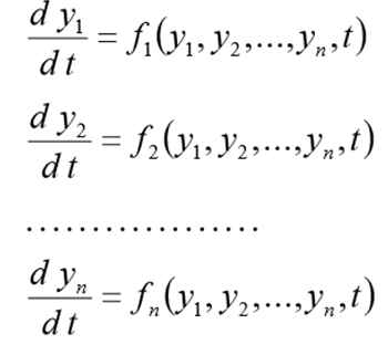
(1)
有初始条件
 Scipy.integrate模块
该模块具有ode()和odeint()两个函数,这些函数设计为在一个点具有初始条件的情况下解决一阶常微分方程(ODE)系统(Cauchy问题)。 ode()函数更通用,而odeint()(ODE积分器)函数具有更简单的界面,可以很好地解决大多数问题。
Odeint()函数odeint()函数具有三个必需的参数和许多选项。 它具有以下格式odeint(func,y0,t [,args =(),...])参数func是两个变量的函数的Python名称,其中第一个是列表y = [y1,y2,...,yn ],第二个是自变量的名称。
Func函数应返回n个函数值的列表
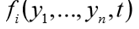
对于独立参数t的给定值。 实际上,func(y,t)函数实现了系统(1)右侧的计算。
odeint()的第二个参数y0是初始值的数组(或列表)
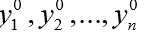
在t = t0时。
第三个参数是要解决问题的时间点数组。 在这种情况下,该数组的第一个元素被视为t0。
odeint()函数返回大小为len(t)x len(y0)的数组。 odeint()函数具有许多控制其操作的选项。 选项rtol(相对误差)和atol(绝对误差)根据公式确定每个yi值的计算误差ei
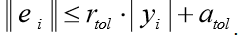
它们可以是向量或标量。 默认情况下
 颂()函数
颂()函数scipy.integrate模块的第二个功能(用于解决微分方程和系统)被称为ode()。 它创建一个ODE对象(类型scipy.integrate._ode.ode)。 与这样一个对象有联系,应该使用其方法来求解微分方程。 与odeint()函数相似,ode(func)函数将问题简化为形式为(1)的微分方程组,并使用其右侧函数。
唯一的区别是右侧func(t,y)的函数接受一个自变量作为第一个参数,而所需函数的值列表作为第二个参数。 例如,以下指令序列将创建一个代表柯西任务的ODE。
龙格-库塔方法在构造数值算法时,我们假设存在对此微分问题的解决方案,它是唯一的并且具有必要的平滑性。
在柯西问题的数值解中
(2)
(3)
根据在点t = 0处的已知解,有必要从公式(3)中找到其他t的解。 在问题(2),(3)的数值解中,为简单起见,我们将在变量t中使用步长t> 0的统一网格。
问题(2),(3)的近似解

表示

。 方法收敛于一点

如果
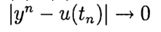
在

。 该方法的精度为p阶
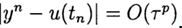
,对于p> 0
。 问题(2),(3)的近似解的最简单差分方案为

(4)
在

我们有一个明确的方法,在这种情况下,差分方案以一阶近似方程(2)。 对称设计

(4)中的方程具有二阶近似。 该方案属于隐式类-要确定新层上的近似解,有必要解决非线性问题。
基于预测器-校正器方法构造显式二阶和高阶逼近方案很方便。 在预测变量(预测)阶段,使用显式方案
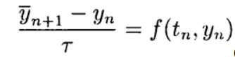
(5)
在校正器(优化)阶段,有一张图
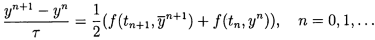
在单步Runge – Kutta方法中,最充分地实现了预测器-校正器的思想。 此方法以一般形式编写:
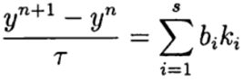
(6)
在哪里
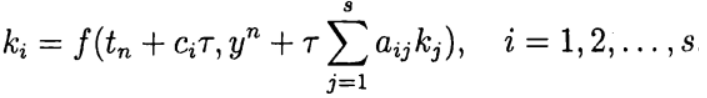
公式(6)基于函数f的s计算,称为s-stage。 如果

在

我们有显式的Runge – Kutta方法。 如果
对于j> 1和

然后

由等式隐式确定:
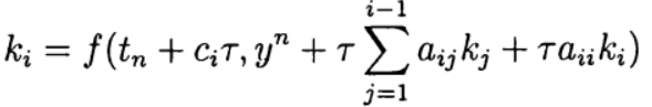
(7)
这种Runge – Kutta方法被称为对角隐式方法。 参量

确定Runge – Kutta方法的变体。 使用以下方法表示(Butcher表)
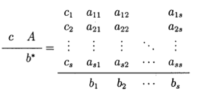
最常见的方法之一是四阶显式Runge – Kutta方法。
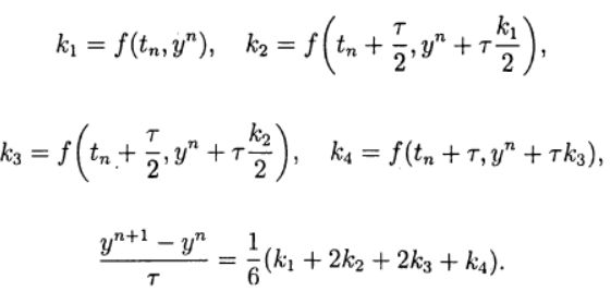
(8)
龙格-库塔-费尔伯格方法我给出计算系数的值
方法

(9)
鉴于(9),一般解的形式为:
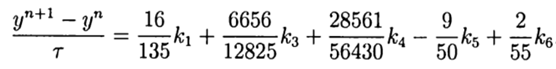
(10)
该解决方案提供了第五个精度等级,仍然可以使其适应Python。
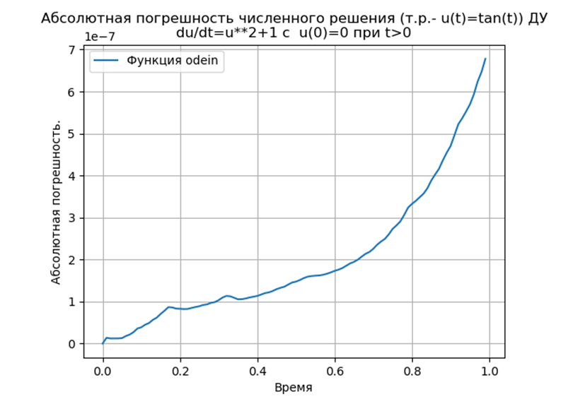
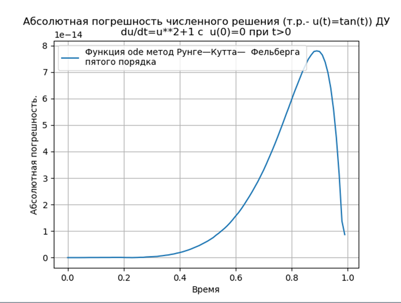
确定非线性微分方程数值解绝对误差的计算实验 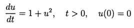 同时使用scipy.integrate模块的def odein()和def oden()函数以及适用于Python的Runge – Kutta和Runge – Kutta – Felberg方法
程序清单from numpy import* import matplotlib.pyplot as plt from scipy.integrate import * def odein():
我们得到:
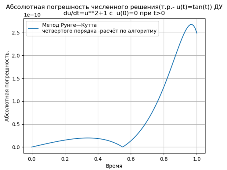
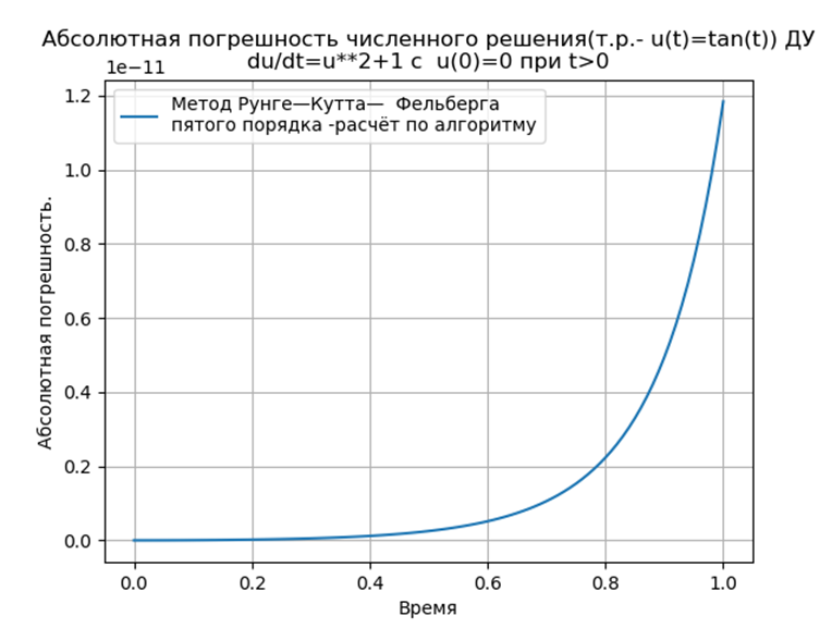
 结论:
结论:与Python匹配的Runge – Kutta和Runge – Kutta – Felberg方法的绝对值比使用odeint函数的解决方案低,但比使用edu函数的解决方案低。 有必要进行性能研究。
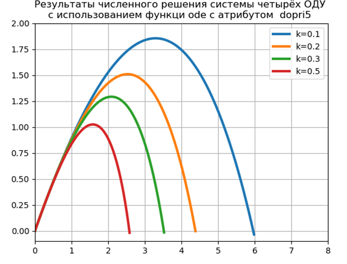
进行数值实验,比较使用ode函数和dopri5属性(五阶Runge – Kutta方法)和使用适用于Python的Runge – Kutta – Felberg方法对SDE进行数值求解的速度
以[2]中给出的模型问题为例进行比较分析。 为了不重复其来源,我将介绍[2]中模型问题的表述和解决方案。
让我们解决柯西问题,该问题描述了在空气阻力与速度的平方成比例的假设下,以初始速度v0投掷物体的运动,该物体相对于地平线成角度α。 在矢量形式中,运动方程的形式为
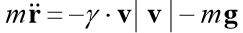
在哪里

是运动物体的矢量的半径,

是身体的速度向量,

-阻力系数,矢量

质量体重的力m,g-重力加速度。
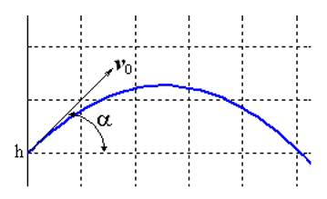
这项任务的特殊性在于,当人体跌落到地面时,运动会在以前未知的时间点结束。 如果指定

,然后以坐标形式有一个方程组:
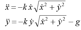
初始条件应添加到系统中:
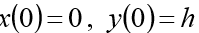
(h初始高度)

。 放
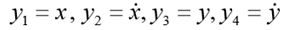
。 然后相应的一阶ODE系统采用以下形式:
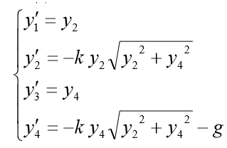
对于模型问题,我们提出

。 省略了对该程序的相当广泛的描述,我将仅从注释中列出一个清单,我认为该清单的操作原理将很清楚。 该程序添加了一个倒计时用于比较分析。
程序清单 import numpy as np import matplotlib.pyplot as plt import time start = time.time() from scipy.integrate import ode ts = [ ] ys = [ ] FlightTime, Distance, Height =0,0,0 y4old=0 def fout(t, y):
我们得到:
飞行时间= 1.2316距离= 5.9829高度= 1.8542
飞行时间= 1.1016距离= 4.3830高度= 1.5088
飞行时间= 1.0197距离= 3.5265高度= 1.2912
飞行时间= 0.9068距离= 2.5842高度= 1.0240
模型出现问题的时间:0.454787
为了在不使用特殊模块的情况下使用Python工具实现CDS的数值解决方案,我提出并研究了以下函数:
def increment(f, t, y, tau
k1=tau*f(t,y)
k2=tau*f(t+(1/4)*tau,y+(1/4)*k1)
k3 =tau *f(t+(3/8)*tau,y+(3/32)*k1+(9/32)*k2)
k4=tau*f(t+(12/13)*tau,y+(1932/2197)*k1-(7200/2197)*k2+(7296/2197)*k3)
k5=tau*f(t+tau,y+(439/216)*k1-8*k2+(3680/513)*k3 -(845/4104)*k4)
k6=tau*f(t+(1/2)*tau,y-(8/27)*k1+2*k2-(3544/2565)*k3 +(1859/4104)*k4-(11/40)*k5)
return (16/135)*k1+(6656/12825)*k3+(28561/56430)*k4-(9/50)*k5+(2/55)*k6
增量(f,t,y,tau)函数提供了数值解法的第五阶。 该程序的其他功能可以在下面的清单中找到:
程序清单 from numpy import* import matplotlib.pyplot as plt import time start = time.time() def rungeKutta(f, to, yo, tEnd, tau): def increment(f, t, y, tau):
我们得到:
模型出现问题的时间:0.259927
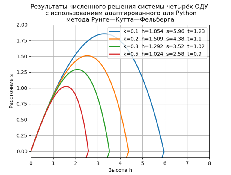 结论
结论在不使用特殊模块的情况下,模型问题的拟议软件实现几乎比使用ode函数具有快两倍的性能,但是我们不能忘记ode具有更高的数值解精度和选择解法的可能性。
用线程分隔的边界条件解决边界值问题
我们以线程分隔的边界条件为例,说明一个特定的边值问题:
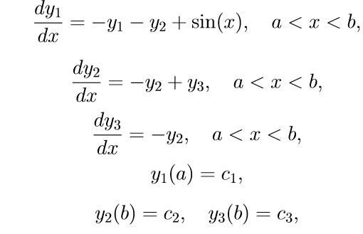
(11)
为了解决问题(11),我们使用以下算法:
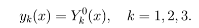
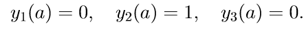
我们用初始条件求解系统(11)的前三个非齐次方程

我们介绍解决柯西问题的符号:
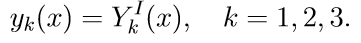
2.用初始条件求解系统(11)的前三个齐次方程
我们介绍解决柯西问题的符号:
3.用初始条件求解系统(11)的前三个齐次方程

我们介绍解决柯西问题的符号:

4.使用柯西问题的解对边值问题的一般解(11)写为解的线性组合:

其中p2,p3是一些未知参数。
5.为了确定参数p2,p3,我们使用最后两个方程式(11)的边界条件,即x = b的条件。 代入,我们得到关于未知p2,p3的线性方程组:
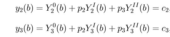
(12)
求解(12),我们得到p2,p3的关系。
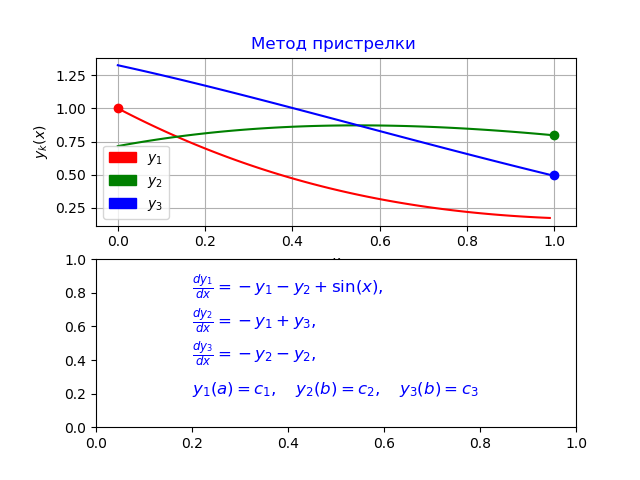
使用以上使用Runge – Kutta – Felberg方法的算法,我们获得以下程序:
我们得到:
y0 [0] = 0.0
y1 [0] = 1.0
y2 [0] = 0.7156448588231397
y3 [0] = 1.324566562303714
y0 [N-1] = 0.9900000000000007
y1 [N-1] = 0.1747719838716767
y2 [N-1] = 0.8
y3 [N-1] = 0.5000000000000001
模型出现问题的时间:0.070878
结论
我开发的程序不同于[3]中给出的错误,该错误证实了本文开头使用python中实现的Runge – Kutta – Felberg方法对odeint函数进行的比较分析。
参考文献:
1.
由微分方程的复合系统定义的对象数学模型的数值解。2.
科学Python简介。3. N.M. E.V. Polyakova Shiryaeva Python 3.创建图形用户界面(使用通过射击方法解决线性常微分方程的边值问题的示例)。 顿河畔罗斯托夫2017。