🤐 📲 🧒🏾 使用SymPy的Laplace变换方法对线性微分方程和系统的符号解 👆🏽 💾 👰🏻

使用符号计算在Python中实现算法对于解决由微分方程定义的对象的数学建模问题非常方便。为了求解这样的方程式，拉普拉斯变换被广泛使用，以简化的术语，这使得可以减少求解简单的代数方程式的问题。

在本出版物中，我建议考虑使用SymPy库中的直接和逆向Laplace变换的功能，这些函数允许您使用Laplace方法来使用Python求解微分方程和系统。

拉普拉斯方法本身及其在求解线性微分方程和系统方面的优势已在文献中广泛报道，例如，在流行的出版物中[1]。在本书中，作者使用选定的示例介绍了Laplace方法，以在许可的软件包Mathematica，Maple和MATLAB中实现该方法（这意味着教育机构购买了该软件）。

今天，我们将尝试考虑的不是使用Python解决学习问题的单独示例，而是考虑使用正向和逆向Laplace变换函数求解线性微分方程和系统的通用方法。同时，我们将节省学习时间：具有考奇条件的线性微分方程的左侧将由学生本人形成，而该任务的例程部分将由laplace_transform（）函数执行，包括方程右侧的直接Laplace变换。

拉普拉斯著作权的故事改变了

拉普拉斯变换（拉普拉斯图像）具有有趣的历史。 L. Euler的作品中第一次出现了确定拉普拉斯变换的积分。但是，数学上通常接受将一种方法或定理称为在欧拉之后发现它的数学家的名字。否则，将有数百种不同的欧拉定理。

在这种情况下，紧随欧拉之后的是法国数学家皮埃尔·西蒙·德拉普拉斯（Pierre Simon de Laplace（1749-1827））。正是他在概率论研究中使用了此类积分。拉普拉斯本人并没有应用所谓的“运算方法”来基于拉普拉斯变换（拉普拉斯图像）找到微分方程的解。这些方法实际上是由实际工程师发现并推广的，特别是英国电气工程师Oliver Heaviside（1850-1925）。尽管这些方法的合法性甚至在20世纪初就受到了很大的质疑，但在严格证明这些方法的有效性的很久之前，运算演算就已经成功地得到了广泛的应用，并且对此话题的争论非常激烈。

拉普拉斯正反变换的功能

拉普拉斯直接转换功能：
sympy.integrals.transforms。 laplace_transform （t，s，**提示）。
laplace_transform（）函数执行实变量的函数f（t）到复杂变量的函数F（s）的Laplace变换，以便：
$F（s）= \ int_ {0} ^ {∞} f（t）e ^ {-st} dt。$

此函数返回（F，a，cond） ，其中F（s）是函数f（t）的拉普拉斯变换， a <Re （s）是定义F（s）的半平面， cond是积分收敛的辅助条件。
如果不能以闭合形式计算积分，则此函数返回未计算的LaplaceTransform对象。
如果设置选项noconds = True ，则该函数仅返回F（s） 。
拉普拉斯逆变换函数：

sympy.integrals.transforms。 inverse_laplace_transform （F，s，t，plane = None，**提示）。

inverse_laplace_transform（）函数执行将复杂变量F（s）的函数转换为实变量的函数f（t）的拉普拉斯逆变换，从而：
$f（t）= \ frac {1} {2 \ pi i} \ int_ {c-∞\ cdot i} ^ {c +∞\ cdot i} e ^ {st} F（s）ds。$

如果无法以闭合形式计算积分，则此函数返回对象的未调用的InverseLaplaceTransform 。

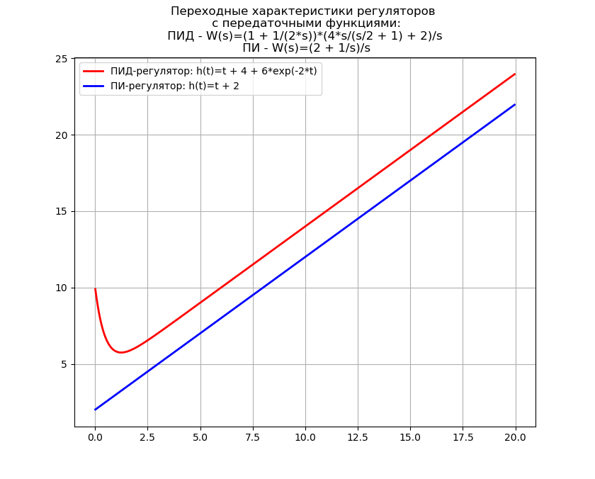
以拉普拉斯逆变换为例确定调节器的过渡特性

PID控制器的传递函数的格式为[2]：

$W（s）=（1+ \ frac {K_ {d} \ cdot T_ {d} \ cdot s} {1 + T_ {d} \ cdot s}）\ cdot K_ {p} \ cdot（1+ \ frac {1} {T_ {i} \ cdot s}）\ cdot \ frac {1} {s}$

我们将编写一个程序，以获取用于简化传递函数的PID和PI控制器瞬态特性的方程式，并另外得出花在逆视觉Laplace变换上的时间。

程序文字

#   : from sympy import * import time import matplotlib.pyplot as plt import numpy as np start = time.time() #   : var('s Kp Ti Kd Td') #      : var('t', positive=True) Kp = 2 Ti = 2 Kd = 4 Td = Rational(1, 2) #   -   s: fp = (1 + (Kd * Td * s) / (1 + Td*s)) * Kp * (1 + 1/(Ti*s)) * (1/s) #   -, #     : ht = inverse_laplace_transform(fp, s, t) Kd = 0 #   - (Kd = 0)   s: fpp = (1 + (Kd * Td * s) / (1 + Td*s)) * Kp * (1 + 1/(Ti*s)) * (1/s) #   -, #     : htt = inverse_laplace_transform(fpp, s, t) stop = time.time() print ('     : %ss' % N((stop-start), 3)) #      : f = lambdify(t, ht, 'numpy') F = lambdify(t, htt, 'numpy') tt = np.arange(0.01, 20, 0.05) #  : plt.title('   \n   : \n  - W(s)=%s \n  - W(s)=%s' % (fp, fpp)) plt.plot(tt, f(tt), color='r', linewidth=2, label='-: h(t)=%s' % ht) plt.plot(tt, F(tt), color='b', linewidth=2, label='-: h(t)=%s' % htt) plt.grid(True) plt.legend(loc='best') plt.show()

我们得到：

反向视觉拉普拉斯变换时间：2.68 s

拉普拉斯逆变换通常用于自行火炮的合成中，在Python中Python可以代替昂贵的软件“怪物”（如MathCAD），因此上述逆变换的使用具有实际意义。

从高阶导数进行拉普拉斯变换以解决柯西问题

我们的讨论将继续使用拉普拉斯变换（拉普拉斯图像）来搜索具有以下常数系数的线性微分方程的解：

$a \ cdot x''（t）+ b \ cdot x'（t）+ c \ cdot x（t）= f（t）。（1）美$

如果a和b是常数，则

$L \左\ {a \ cdot f（t）+ b \ cdot q（t）\右\} = a \ cdot L \左\ {f（t）\右\} + b \ cdot L \左\ {q（t）\ right \}（2）$

对于所有s ，函数f（t）和q（t）的两个Laplace变换（Laplace图像）都存在。

让我们使用先前考虑的函数laplace_transform（）和inverse_laplace_transform（）来验证正拉普拉斯变换和逆拉普拉斯变换的线性。为此，我们以f（t）= sin（3t） ， q（t）= cos（7t） ， a = 5 ， b = 7为例，并使用以下程序。

程序文字

 from sympy import* var('sa b') var('t', positive=True) a = 5 f = sin(3*t) b = 7 q = cos(7*t) #   a*L{f(t)}: L1 = a * laplace_transform(f, t, s, noconds=True) #   b*L{q(t)}: L2 = b*laplace_transform(q, t, s, noconds=True) #  a*L{f(t)}+b*L{q(t)}: L = factor(L1 + L2) print (L) #   L{a*f(t)+b*q(t)}: LS = factor(laplace_transform(a*f + b*q, t, s, noconds=True)) print (LS) print (LS == L) #   a* L^-1{f(t)}: L_1 = a * inverse_laplace_transform(L1/a, s, t) #   b* L^-1{q(t)} L_2 = b * inverse_laplace_transform(L2/b, s, t) # a* L^-1{f(t)}+b* L^-1{q(t)}: L_S = L_1 + L_2 print (L_S) #   L^-1{a*f(t)+b*q(t)}: L_1_2 = inverse_laplace_transform(L1 + L2, s, t) print (L_1_2) print (L_1_2 == L_S)

我们得到：

（7 * s ** 3 + 15 * s ** 2 + 63 * s + 735）/（（s ** 2 + 9）*（s ** 2 + 49））
（7 * s ** 3 + 15 * s ** 2 + 63 * s + 735）/（（s ** 2 + 9）*（s ** 2 + 49））
是的
5 *罪（3 * t）+ 7 * cos（7 * t）
5 *罪（3 * t）+ 7 * cos（7 * t）

上面的代码还演示了拉普拉斯逆变换的唯一性。

假设

$q（t）= f'（t）$ 满足第一个定理的条件，则从该定理中可以得出：

$L \左\ {f''（t）\右\} = L \左\ {q'（t）\右\} = sL \左\ {q（t）\右\}-q（0） = sL \左\ {f'（t）\右\}-f'（0）= s \左[sL \左\ {f（t）-f（0）\右\} \右]，$

因此

$L \左\ {f''（t）\右\} = s ^ {2} \ cdot F（s）-s \ cdot f（0）-f'（0）。$

重复此计算，得出

$L \左\ {f'''（t）\右\} = sL \左\ {f''（t）\右\}-f''（0）= s ^ {3} F（s） -s ^ {2} f（0）-sf'（0）-f''（0）。$

经过有限数量的这样的步骤，我们得到第一个定理的以下概括：

$L \左\ {f ^ {{n}}（t）\右\} = s ^ {n} L \左\ {f（t）\右\}-s ^ {n-1} f（0 ）-s ^ {n-2} f'（0）-\ cdot \ cdot \ cdot -f ^ {（n-1）}（0）=$

$= s ^ {n} F（s）-s ^ {n-1} f（0）-\ cdot \ cdot \ cdot -sf ^ {（n-2）}（0）-f ^ {（n- 1）}（0）。（3）美$

将关系式（3）（包含具有初始条件的所需函数的经拉普拉斯变换的导数）应用于方程式（1），我们可以根据我们部门专门开发的方法在Scorobey的SymPy库的积极支持下获得其解决方案。

SymPy库基于Laplace变换的线性微分方程和方程组的求解方法

为了演示该方法，我们使用一个简单的微分方程来描述由给定质量的材料点组成的系统的运动，该系统安装在施加外力的弹簧上。该系统的微分方程和初始条件具有以下形式：

$x''+ 4x = \ sin（3吨）; x（0）= 1.2； x'（0）= 1，（4）$

在哪里

$x（0）$ -减少质量的初始位置，

$x'（0）$ -降低初始质量速度。

由等式（4）定义的简化物理模型，初始条件为非零[1]：

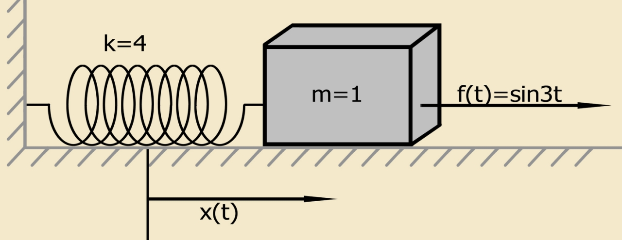
由固定在弹簧上的给定质量的物质点组成的系统满足柯西问题（初始条件问题）。给定质量的物质点最初在其平衡位置处于静止状态。

为了通过拉普拉斯变换法求解该线性方程和其他线性微分方程，使用从关系式（3）获得的以下系统很方便：

$L \左\ {f ^ {IV}（t）\右\} = s ^ {4} \ cdot F（s）-s ^ {3} \ cdot f（0）-s ^ {2} \ cdot f ^ {I}（0）-s \ cdot f ^ {II}（0）-f ^ {III}（0），$

$L \左\ {f ^ {III}（t）\右\} = s ^ {3} \ cdot f（s）-s ^ {2} \ cdot f（0）-s \ cdot f ^ {I }（0）-f ^ {II}（0），$

$L \左\ {f ^ {II}（t）\右\} = s ^ {2} \ cdot F（s）-s \ cdot f（0）-f ^ {I}（0），$

$L \左\ {f ^ {I}（t）\右\} = s \ cdot F（s）-f（0），L \左\ {f（t）\右\} = F（s）$

$L \左\ {f（t）\右\} = F（s）。（5）$

使用SymPy的解决方案的顺序如下：

加载必要的模块并显式定义符号变量：

 from sympy import * import numpy as np import matplotlib.pyplot as plt var('s') var('t', positive=True) var('X', cls=Function)

指定sympy库的版本以考虑其功能。为此，请输入以下行：
```
 import SymPy print ('  sympy – %' % (sympy._version_)) 
```
根据问题的物理含义，为包含零和正数的区域确定时间变量。我们在方程式（4）的右侧及其后续的Laplace变换中设置初始条件和函数。对于初始条件，必须使用Rational函数，因为使用十进制舍入会导致错误。
```
 #    : x0 = Rational(6, 5) #   : x01 = Rational(1, 1) g = sin(3*t) Lg = laplace_transform(g, t, s, noconds=True) 
```
使用（5），我们重写方程式（4）左侧包含的经Laplace转换的导数，从它们构成该方程式的左侧，并将结果与其右侧进行比较：
```
 d2 = s**2*X(s) - s*x0 - x01 d0 = X(s) d = d2 + 4*d0 de = Eq(d, Lg) 
```
我们为变换X（s）求解获得的代数方程，并执行拉普拉斯逆变换：
```
 rez = solve(de, X(s))[0] soln = inverse_laplace_transform(rez, s, t) 
```
我们从SymPy库中的工作转移到NumPy库中：
```
 f = lambdify(t, soln, 'numpy') 
```

我们绘制了常用的Python方法：

 x = np.linspace(0, 6*np.pi, 100) plt.title(',     \n  :\n  (t)=%s' % soln) plt.grid(True) plt.xlabel('t', fontsize=12) plt.ylabel('x(t)', fontsize=12) plt.plot(x, f(x), 'g', linewidth=2) plt.show()

程序全文：

 from sympy import * import numpy as np import matplotlib.pyplot as plt import sympy var('s') var('t', positive=True) var('X', cls=Function) print ("  sympy – %s" % (sympy.__version__)) #       : x0 = Rational(6, 5) #       : x01 = Rational(1, 1) g = sin(3*t) #   : Lg = laplace_transform(g, t, s, noconds=True) d2 = s**2*X(s) - s*x0 - x01 d0 = X(s) d = d2 + 4*d0 de = Eq(d, Lg) #   : rez = solve(de, X(s))[0] #   : soln = inverse_laplace_transform(rez, s, t) f = lambdify(t, soln, "numpy") x = np.linspace(0, 6*np.pi, 100) plt.title(',     \n  :\n  (t)=%s' % soln) plt.grid(True) plt.xlabel('t', fontsize=12) plt.ylabel('x(t)', fontsize=12) plt.plot(x, f(x), 'g', linewidth=2) plt.show()

我们得到：
Sympy库版本-1.3

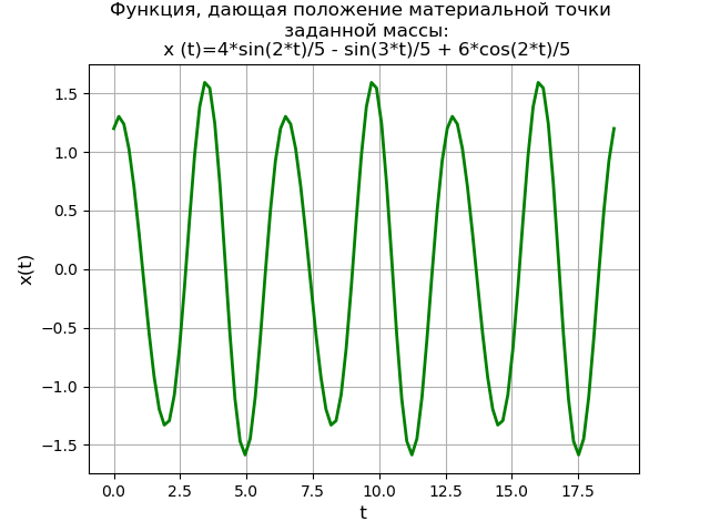
获得给出给定质量的物质点位置的周期函数图。使用SymPy库的Laplace变换方法不仅提供解决方案，而且无需首先找到齐次方程的通用解和初始的非均质微分方程的特定解，而且还不需要使用基本分数法和Laplace表。

同时，由于需要使用系统（5），因此保留了求解方法的教育价值，并前往NumPy使用更高效的方法来研究求解。

为了进一步说明该方法，我们解决了微分方程组：

$\开始{cases} 2x''+ 6x-2 = 0，\\ y''-2x + 2y = 40 \ cdot \ sin（3t），\ end {cases（6）$
有初始条件

$x（0）= y（0）= y'（0）= 0$

在零初始条件下由方程式（6）的系统定义的简化物理模型：

因此，当系统在其平衡位置静止时，在时间t = 0时，力f（t）突然施加到给定质量的第二个物质点。

方程组的解与之前考虑的微分方程（4）的解相同，因此，我在不做解释的情况下给出了程序文本。

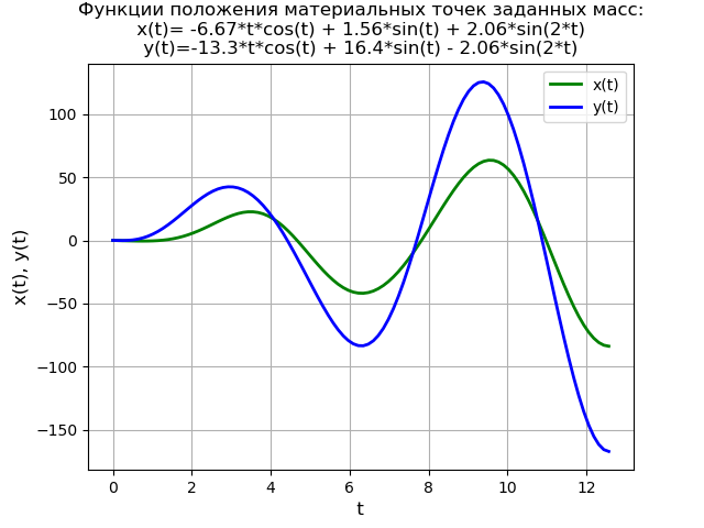
程序文字

 from sympy import * import numpy as np import matplotlib.pyplot as plt var('s') var('t ', positive=True) var('X Y', cls=Function) x0 = 0 x01 = 0 y0 = 0 y01 = 0 g = 40 * sin(3*t) Lg = laplace_transform(g, t, s, noconds=True) de1 = Eq(2*(s**2*X(s) - s*x0 - x01) + 6*X(s) - 2*Y(s)) de2 = Eq(s**2*Y(s) - s*y0 - y01 - 2*X(s) + 2*Y(s) - Lg) rez = solve([de1, de2], X(s), Y(s)) rezX = expand(rez[X(s)]) solnX = inverse_laplace_transform(rezX, s, t) rezY = expand(rez[Y(s)]) solnY = inverse_laplace_transform(rezY, s, t) f = lambdify(t, solnX, "numpy") F = lambdify(t, solnY, "numpy") x = np.linspace(0, 4*np.pi, 100) plt.title('     :\nx(t)=%s\ny(t)=%s' % (solnX, solnY)) plt.grid(True) plt.xlabel('t', fontsize=12) plt.ylabel('x(t), y(t)', fontsize=12) plt.plot(x, f(x), 'g', linewidth=2, label='x(t)') plt.plot(x, F(x), 'b', linewidth=2, label='y(t)') plt.legend(loc='best') plt.show()

我们得到：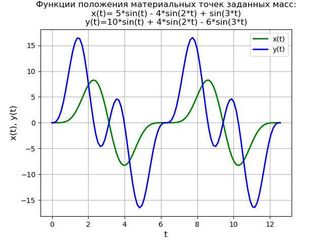

对于非零初始条件，程序文本和功能图将采用以下形式：

程序文字

 from sympy import * import numpy as np import matplotlib.pyplot as plt var('s') var('t', positive=True) var('X Y', cls=Function) x0 = 0 x01 = -1 y0 = 0 y01 = -1 g = 40 * sin(t) Lg = laplace_transform(g, t, s, noconds=True) de1 = Eq(2*(s**2*X(s) - s*x0 - x01) + 6*X(s) - 2*Y(s)) de2 = Eq(s**2*Y(s) - s*y0 - y01 - 2*X(s) + 2*Y(s) - Lg) rez = solve([de1, de2], X(s), Y(s)) rezX = expand(rez[X(s)]) solnX = (inverse_laplace_transform(rezX, s, t)).evalf().n(3) rezY = expand(rez[Y(s)]) solnY = (inverse_laplace_transform(rezY, s, t)).evalf().n(3) f = lambdify(t, solnX, "numpy") F = lambdify(t, solnY, "numpy") x = np.linspace(0, 4*np.pi, 100) plt.title('     :\nx(t)= %s \ny(t)=%s' % (solnX, solnY)) plt.grid(True) plt.xlabel('t', fontsize=12) plt.ylabel('x(t), y(t)', fontsize=12) plt.plot(x, f(x), 'g', linewidth=2, label='x(t)') plt.plot(x, F(x), 'b', linewidth=2, label='y(t)') plt.legend(loc='best') plt.show()

考虑初始条件为零的四阶线性微分方程的解：

$x ^ {（4）} + 2 \ cdot x''+ x = 4 \ cdot t \ cdot e ^ {t};$

$x（0）= x'（0）= x''（0）= x ^ {（3）}（0）= 0$

程序文字：

 from sympy import * import numpy as np import matplotlib.pyplot as plt var('s') var('t', positive=True) var('X', cls=Function) #  : x0 = 0 x01 = 0 x02 = 0 x03 = 0 g = 4*t*exp(t) #   : Lg = laplace_transform(g, t, s, noconds=True) d4 = s**4*X(s) - s**3*x0 - s**2*x01 - s*x02 - x03 d2 = s**2*X(s) - s*x0 - x01 d0 = X(s) d = factor(d4 + 2*d2 + d0) de = Eq(d, Lg) #   : rez = solve(de, X(s))[0] #   : soln = inverse_laplace_transform(rez, s, t) f = lambdify(t, soln, "numpy") x = np.linspace(0, 6*np.pi, 100) plt.title(':\n  (t)=%s\n' % soln, fontsize=11) plt.grid(True) plt.xlabel('t', fontsize=12) plt.ylabel('x(t)', fontsize=12) plt.plot(x, f(x), 'g', linewidth=2) plt.show()

决策时间表：

我们求解四阶线性微分方程：

$x ^ {（4）} + 13x''+ 36x = 0;$
有初始条件

$x（0）= x''（0）= 0$ ，

$x'（0）= 2$ ，

$x ^ {（3）}（0）=-13$ 。

程序文字：

 from sympy import * import numpy as np import matplotlib.pyplot as plt var('s') var('t', positive=True) var('X', cls=Function) #  : x0 = 0 x01 = 2 x02 = 0 x03 = -13 d4 = s**4*X(s) - s**3*x0 - s**2*x01 - s*x02 - x03 d2 = s**2*X(s) - s*x0 - x01 d0 = X(s) d = factor(d4 + 13*d2 + 36*d0) de = Eq(d, 0) #   : rez = solve(de, X(s))[0] #   : soln = inverse_laplace_transform(rez, s, t) f = lambdify(t, soln, "numpy") x = np.linspace(0, 6*np.pi, 100) plt.title(':\n  (t)=%s\n' % soln, fontsize=11) plt.grid(True) plt.xlabel('t', fontsize=12) plt.ylabel('x(t)', fontsize=12) plt.plot(x, f(x), 'g', linewidth=2) plt.show()

决策时间表：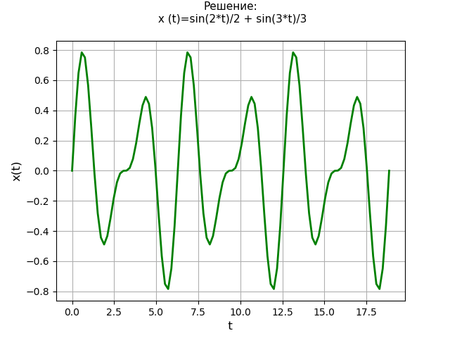

解决ODE的功能

对于具有解析解决方案的ODE和ODE系统，使用dsolve（）函数：
sympy.solvers.ode。 dsolve （eq，func =无，提示='默认'，简化= True，ics =无，xi =无，eta =无，x0 = 0，n = 6，** kwargs）

让我们将dsolve（）函数与Laplace方法的性能进行比较。例如，采用以下初始条件为零的四阶微分方程：

$x ^ {{IV）}（t）= 3 \ cdot x'''（t）-x（t）= 4 \ cdot t \ cdot \ exp（t）;$

$x（0）= x'（0）= x''（0）= x'''（0）= 0.$

一个使用dsolve（）函数的程序：

 from sympy import * import time import numpy as np import matplotlib.pyplot as plt start = time.time() var('t C1 C2 C3 C4') u = Function("u")(t) #   : de = Eq(u.diff(t, t, t, t) - 3*u.diff(t, t, t) + 3*u.diff(t, t) - u.diff(t), 4*t*exp(t)) #   : des = dsolve(de, u) #  : eq1 = des.rhs.subs(t, 0) eq2 = des.rhs.diff(t).subs(t, 0) eq3 = des.rhs.diff(t, t).subs(t, 0) eq4 = des.rhs.diff(t, t, t).subs(t, 0) #       : seq = solve([eq1, eq2-1, eq3-2, eq4-3], C1, C2, C3, C4) rez = des.rhs.subs([(C1, seq[C1]), (C2, seq[C2]), (C3, seq[C3]), (C4, seq[C4])]) def F(t): return rez f = lambdify(t, rez, 'numpy') x = np.linspace(0, 6*np.pi, 100) stop = time.time() print ('      dsolve(): %ss' % round((stop-start), 3)) plt.title('    dsolve():\n  (t)=%s\n' % rez, fontsize=11) plt.grid(True) plt.xlabel('Time t seconds', fontsize=12) plt.ylabel('f(t)', fontsize=16) plt.plot(x, f(x), color='#008000', linewidth=3) plt.show()

我们得到：

使用dsolve（）函数的方程时间：1.437 s

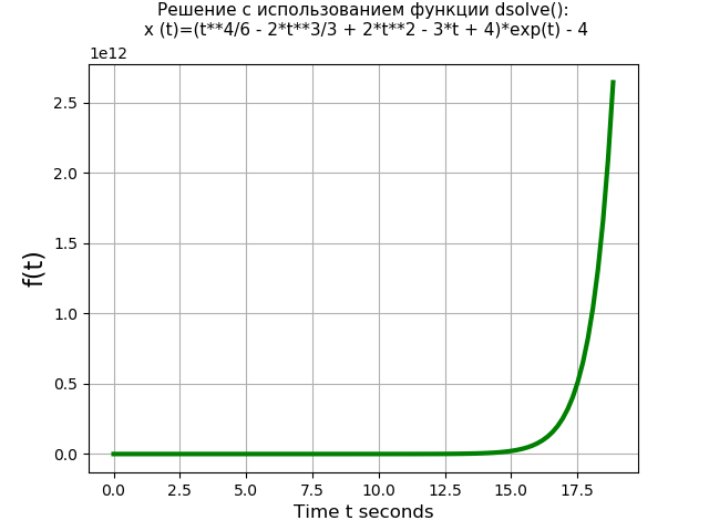
使用Laplace变换的程序：

 from sympy import * import time import numpy as np import matplotlib.pyplot as plt start = time.time() var('s') var('t', positive=True) var('X', cls=Function) #  : x0 = 0 x01 = 0 x02 = 0 x03 = 0 #     : g = 4*t*exp(t) #   : Lg = laplace_transform(g, t, s, noconds=True) d4 = s**4*X(s) - s**3*x0 - s**2*x01 - s*x02 - x03 d3 = s**3*X(s) - s**2*x0 - s*x01 - x02 d2 = s**2*X(s) - s*x0 - x01 d1 = s*X(s) - x0 d0 = X(s) #     : d = factor(d4 - 3*d3 + 3*d2 - d1) de = Eq(d, Lg) #   : rez = solve(de, X(s))[0] #   : soln = collect(inverse_laplace_transform(rez, s, t), t) f = lambdify(t, soln, 'numpy') x = np.linspace(0, 6*np.pi, 100) stop = time.time() print ('      : %ss' % round((stop-start), 3)) plt.title('    :\n  (t)=%s\n' % soln, fontsize=11) plt.grid(True) plt.xlabel('t', fontsize=12) plt.ylabel('x(t)', fontsize=12) plt.plot(x, f(x), 'g', linewidth=2) plt.show()

我们得到：

使用Laplace变换的方程时间：3.274 s

因此，dsolve（）函数（1.437 s）求解四阶方程的速度比通过Laplace变换方法（3.274 s）求解的速度快两倍以上。但是，应注意，dsolve（）函数不能求解二阶微分方程组，例如，当使用dsolve（）函数求解系统（6）时，会发生错误：

 from sympy import* t = symbols('t') x, y = symbols('x, y', Function=True) eq = (Eq(Derivative(x(t), t, 2), -3*x(t) + y(t)), Eq(Derivative(y(t), t, 2), 2*x(t) - 2*y(t) + 40*sin(3*t))) rez = dsolve(eq) print (list(rez))

我们得到：

raiseNotImplementedError
NotImplementedError

此错误意味着使用dsolve（）函数的微分方程组的解不能用符号表示。借助于Laplace变换，我们得到了该解决方案的符号表示，这证明了所提方法的有效性。

注意事项

为了找到使用dsolve（）函数求解微分方程的必要方法，您需要使用classify_ode（eq，f（x）） ，例如：

 from sympy import * from IPython.display import * import matplotlib.pyplot as plt init_printing(use_latex=True) x = Symbol('x') f = Function('f') eq = Eq(f(x).diff(x, x) + f(x), 0) print (dsolve(eq, f(x))) print (classify_ode(eq, f(x))) eq = sin(x)*cos(f(x)) + cos(x)*sin(f(x))*f(x).diff(x) print (classify_ode(eq, f(x))) rez = dsolve(eq, hint='almost_linear_Integral') print (rez)

我们得到：

方程（f（x），C1 * sin（x）+ C2 * cos（x））
（“ nth_linear_constant_coeff_homogeneous”，“ 2nd_power_series_ordinary”）
（“可分离”，“ 1精确”，“几乎线性”，“ 1功率系列”，“谎言组”，“可分离积分”，“ 1精确精确积分”，“几乎线性整体”）
[Eq（f（x），-acos（（C1 +积分（0，x））* exp（-积分（-tan（x），x）））+ 2 * pi），Eq（f（x）， acos（（C1 +积分（0，x））* exp（-积分（-tan（x），x）））]]

因此，对于等式eq = Eq（f（x）.diff（x，x）+ f（x），0） ，第一个列表中的任何方法均有效：

nth_linear_constant_coeff_homogeneous，
2nd_power_series_ordinary

对于方程eq = sin（x）* cos（f（x））+ cos（x）* sin（f（x））* f（x）.diff（x） ，第二个列表中的任何方法均有效：

可分离，精确的，线性的，
1st_power_series，lie_group，separate_Integral，
1st_exact_Integral，几乎_linear_Integral

要使用所选方法，dsolve（）函数条目将采用以下形式：

 rez = dsolve(eq, hint='almost_linear_Integral')

结论：

本文旨在通过使用算子方法求解线性ODE系统的示例，说明如何使用SciPy和NumPy库的工具。因此，考虑了使用Laplace方法的线性微分方程的符号解方法和方程组。对这种方法以及在dsolve（）函数中实现的方法进行了性能分析。

参考文献：

微分方程和边值问题：使用Mathematica，Maple和MATLAB进行建模和计算。第三版。来自英语 -M .: LLC“ I.D. 威廉姆斯（Williams），2008年。-1104羽。 -Paral。山雀。英文
使用拉普拉斯逆变换来分析控制系统的动态链接

使用SymPy的Laplace变换方法对线性微分方程和系统的符号解

拉普拉斯著作权的故事改变了

拉普拉斯正反变换的功能

以拉普拉斯逆变换为例确定调节器的过渡特性

从高阶导数进行拉普拉斯变换以解决柯西问题

SymPy库基于Laplace变换的线性微分方程和方程组的求解方法

解决ODE的功能

结论：

More articles: