哈Ha! 我向您提供文章“训练您的第一个神经网络:基本分类”的翻译 。

这是用于对运动鞋和衬衫等衣服的图像进行分类的神经网络模型培训指南。 为了创建神经网络,我们使用python和TensorFlow库。
安装TensorFlow
为了工作,我们需要以下库:
- numpy(在命令行我们编写:pip install numpy)
- matplotlib(在命令行我们编写:pip install matplotlib)
- keras(在命令行中,我们编写:pip install keras)
- jupyter(在命令行中我们编写:pip install jupyter)
在命令行上使用pip:编写pip install tensorflow
如果出现错误,则可以下载.whl文件并使用pip进行安装:pip install file_path \ file_name.whl
TensorFlow官方安装指南
启动Jupyter。 要从命令行开始,请编写jupyter notebook。
开始使用
本指南使用Fashion MNIST数据集,其中包含10个类别的70,000张灰度图像。 图像显示了分辨率较低(28 x 28像素)的衣物:

我们将使用60,000张图像来训练网络,并使用10,000张图像来评估网络学会对图像进行分类的准确度。 您只需导入和下载数据即可直接从TensorFlow访问Fashion MNIST:
fashion_mnist = keras.datasets.fashion_mnist (train_images, train_labels), (test_images, test_labels) = fashion_mnist.load_data()
加载数据集将返回四个NumPy数组:
- 数组train_images和train_labels是模型用于训练的数据
- 数组test_images和test_labels用于测试模型。
图片是28x28 NumPy数组,其像素值范围是0到255。标签是0到9的整数数组。它们对应于服装类:
| 标签 | 班级 |
| 0 | T恤(T恤) |
| 1个 | 裤子(裤子) |
| 2 | 套头衫(毛衣) |
| 3 | 着装 |
| 4 | 大衣(大衣) |
| 5 | 凉鞋 |
| 6 | 上衣 |
| 7 | 运动鞋(运动鞋) |
| 8 | 包袋 |
| 9 | 脚踝靴(脚踝靴) |
类名不包含在数据集中,所以我们自己给它开处方:
class_names = ['T-shirt/top', 'Trouser', 'Pullover', 'Dress', 'Coat', 'Sandal', 'Shirt', 'Sneaker', 'Bag', 'Ankle boot']
数据探索
在训练模型之前,请考虑数据集格式。
train_images.shape
数据预处理
在准备模型之前,必须对数据进行预处理。 如果检查训练集中的第一张图像,您将看到像素值在0到255之间:
plt.figure() plt.imshow(train_images[0]) plt.colorbar() plt.grid(False)

我们将这些值缩放为0到1:
train_images = train_images / 255.0 test_images = test_images / 255.0
我们显示训练集中的前25张图像,并在每张图像下方显示班级名称。 确保数据格式正确。
plt.figure(figsize=(10,10)) for i in range(25): plt.subplot(5,5,i+1) plt.xticks([]) plt.yticks([]) plt.grid(False) plt.imshow(train_images[i], cmap=plt.cm.binary) plt.xlabel(class_names[train_labels[i]])

模型制作
建立神经网络需要调整模型的各个层。
神经网络的主要组成部分是层。 大多数深度学习都在于组合简单的层。 大多数图层(例如tf.keras.layers.Dense)具有在训练期间学习的参数。
model = keras.Sequential([ keras.layers.Flatten(input_shape=(28, 28)), keras.layers.Dense(128, activation=tf.nn.relu), keras.layers.Dense(10, activation=tf.nn.softmax) ])
网络tf.keras.layers.Flatten中的第一层将图像格式从2d数组(28 x 28像素)转换为28 * 28 = 784像素的1d数组。 该层没有要研究的参数,仅重新格式化数据。
接下来的两层是tf.keras.layers.Dense。 这些是紧密连接或完全连接的神经层。 第一密集层包含128个节点(或神经元)。 第二(也是最后一个)层是一个包含10个节点tf.nn.softmax的层,该层返回一个包含10个概率估计值的数组,其总和为1。每个节点包含一个估计值,该估计值指示当前图像属于10个类别之一的可能性。
编译模型
在模型准备好进行训练之前,它将需要进行一些其他设置。 它们是在模型的编译阶段添加的:
- 损失函数-测量训练过程中模型的准确性
- Optimizer是基于模型看到的数据和损失函数来更新模型的方法。
- 指标(指标)-用于控制培训和测试的阶段
model.compile(optimizer=tf.train.AdamOptimizer(), loss='sparse_categorical_crossentropy', metrics=['accuracy'])
模型训练
学习神经网络模型需要执行以下步骤:
- 提交模型训练数据(在此示例中,数组train_images和train_labels)
- 模型学习关联图像和标签。
- 我们要求模型对测试套件进行预测(在本示例中为数组test_images)。 我们从标签数组(在本示例中为test_labels数组)检查标签预测的一致性
要开始训练,请调用model.fit方法:
model.fit(train_images, train_labels, epochs=5)
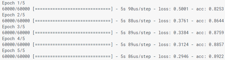
在对模型进行建模时,将显示损失(损耗)和准确性(acc)的指标。 根据训练数据,该模型可实现约0.88(或88%)的精度。
准确度等级
比较模型在测试数据集中的工作方式:
test_loss, test_acc = model.evaluate(test_images, test_labels) print('Test accuracy:', test_acc)
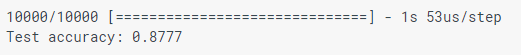
事实证明,测试数据集中的准确性略小于训练数据集中的准确性。 培训准确性和测试准确性之间的差距是再培训的一个示例。 训练是指机器学习模型在使用新数据时比使用训练数据时效果更差的情况。
预测性
我们使用该模型来预测一些图像。
predictions = model.predict(test_images)
在这里,模型预测了测试案例中每个图像的标签。 让我们看一下第一个预测:
predictions[0]
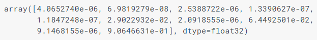
预测是10个数字组成的数组。 他们描述了模型的“置信度”,即图像对应于10种不同衣物的每一种。 我们可以看到哪个标签的置信度最高:
np.argmax(predictions[0])
因此,模型最有信心该图像是脚踝靴(脚踝靴)或class_names [9]。 我们可以检查测试标签以确保正确:
test_labels[0]
我们将编写函数以可视化这些预测。
def plot_image(i, predictions_array, true_label, img): predictions_array, true_label, img = predictions_array[i], true_label[i], img[i] plt.grid(False) plt.xticks([]) plt.yticks([]) plt.imshow(img, cmap=plt.cm.binary) predicted_label = np.argmax(predictions_array) if predicted_label == true_label: color = 'blue' else: color = 'red' plt.xlabel("{} {:2.0f}% ({})".format(class_names[predicted_label], 100*np.max(predictions_array), class_names[true_label]), color=color) def plot_value_array(i, predictions_array, true_label): predictions_array, true_label = predictions_array[i], true_label[i] plt.grid(False) plt.xticks([]) plt.yticks([]) thisplot = plt.bar(range(10), predictions_array, color="#777777") plt.ylim([0, 1]) predicted_label = np.argmax(predictions_array) thisplot[predicted_label].set_color('red') thisplot[true_label].set_color('blue')
让我们看一下第0张图片,预测和预测数组。
i = 0 plt.figure(figsize=(6,3)) plt.subplot(1,2,1) plot_image(i, predictions, test_labels, test_images) plt.subplot(1,2,2) plot_value_array(i, predictions, test_labels)

让我们用它们的预测构建一些图像。 正确的预测标签为蓝色,错误的预测标签为红色。 请注意,即使他很有信心,这也可能是错误的。
num_rows = 5 num_cols = 3 num_images = num_rows*num_cols plt.figure(figsize=(2*2*num_cols, 2*num_rows)) for i in range(num_images): plt.subplot(num_rows, 2*num_cols, 2*i+1) plot_image(i, predictions, test_labels, test_images) plt.subplot(num_rows, 2*num_cols, 2*i+2) plot_value_array(i, predictions, test_labels)

最后,我们使用经过训练的模型对单个图像进行预测。
Tf.keras模型经过优化,可以对包装(批次)或集合(集合)进行预测。 因此,尽管我们使用单个图像,但需要将其添加到列表中:
图片预测:
predictions_single = model.predict(img) print(predictions_single)

plot_value_array(0, predictions_single, test_labels) _ = plt.xticks(range(10), class_names, rotation=45)

np.argmax(predictions_single[0])
和以前一样,该模型将预测标签9。
如有疑问,请在评论中或私人留言中写下。