从零开始编写XGBoost-第2部分：梯度提升

大家好！

在上一篇文章中，我们了解了决策树的排列方式，并从头开始实现
施工算法，同时对其进行优化和改进。 在本文中，我们将实现梯度提升算法，最后，我们将创建自己的XGBoost。 叙述将遵循相同的模式：我们编写一种算法，对其进行描述，然后通过比较使用Sklearn的类似物的结果来总结该算法。

在本文中，还将重点放在代码的实现上，因此最好以另一种形式（例如在ODS课程中 ）一起阅读整个理论，并且已经具备了该理论的知识，您可以继续阅读本文，因为该主题非常复杂。



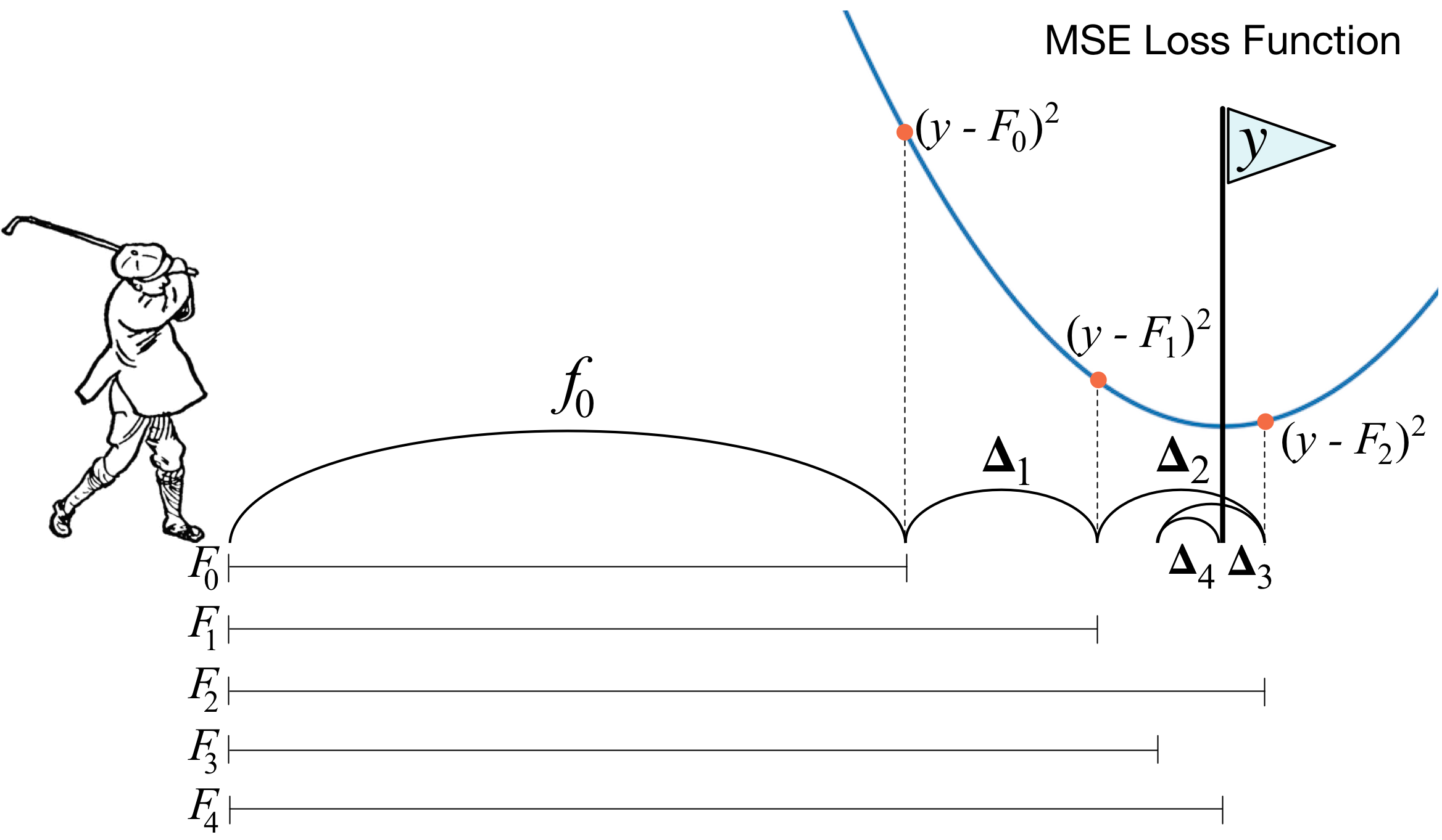
什么是梯度增强？ 高尔夫球手的照片完美地描述了主要思想。 为了将球打入洞中，高尔夫球手在下一次击打时要考虑到先前的击球经验-对他而言，这是将球放入洞中的必要条件。 如果非常不礼貌（我不是高尔夫球高手），那么每次击球时，高尔夫球手首先要看的是击球后球与洞之间的距离。 主要任务是在下一次打击时减小该距离。

提升的建立方式非常相似。 首先，我们需要引入“空洞”的定义，即我们将努力追求的目标。 其次，我们需要学习理解我们需要与哪一方打败才能更接近目标。 第三，考虑所有这些规则，您需要提出正确的击球顺序，以便随后的每个击球都可以减小球与洞之间的距离。

现在我们给出一个更严格的定义。 我们介绍加权投票的模型：

$$

$$h（x）= \ sum_ {i = 1} ^ nb_ia_i，x \ in X，b_i \ in R$$

在这里 $$$X$是我们用来取物的空间， $$$b_i，a_i$-这是模型和模型本身前面的系数，即决策树。 假设已经使用描述的规则在某个步骤中添加了合成 $$$T-1$弱算法。 要学习了解应该采用哪种算法 $$$T$，我们介绍误差函数：

$$$err（h）= \ sum_ {j = 1} ^ N L（\ sum_ {i = 1} ^ {T-1} a_ib_i（x_j）+ b_Ta_T（x_j））\ rightarrow min_ {a_T，b_T}$

事实证明，最好的算法将是可以最小化先前迭代中收到的错误的算法。 并且由于提升是渐变的，因此此误差函数必须必须具有反梯度向量，您可以沿着该向量移动以寻找最小值。 仅此而已！

在即将实施之前，我将添加几句话，说明如何与我们一起安排一切。 与上一篇文章一样，我们将MSE视为损失。 让我们计算它的梯度：

$$

$$mse（y，预测）=（y-预测）^ 2 \\ \ nabla_ {predict} mse（y，预测）=预测-y$$

因此，反梯度向量将等于 $$$y-预测$。 在台阶上 $$$我$我们考虑在先前迭代中获得的算法的错误。 接下来，我们针对这些错误训练新算法，然后使用负号和一些系数将其添加到集合中。

现在开始吧。

1.实现通常的梯度增强类

import pandas as pd import matplotlib.pyplot as plt import numpy as np from tqdm import tqdm_notebook from sklearn import datasets from sklearn.metrics import mean_squared_error as mse from sklearn.tree import DecisionTreeRegressor import itertools %matplotlib inline %load_ext Cython %%cython -a import itertools import numpy as np cimport numpy as np from itertools import * cdef class RegressionTreeFastMse: cdef public int max_depth cdef public int feature_idx cdef public int min_size cdef public int averages cdef public np.float64_t feature_threshold cdef public np.float64_t value cpdef RegressionTreeFastMse left cpdef RegressionTreeFastMse right def __init__(self, max_depth=3, min_size=4, averages=1): self.max_depth = max_depth self.min_size = min_size self.value = 0 self.feature_idx = -1 self.feature_threshold = 0 self.left = None self.right = None def fit(self, np.ndarray[np.float64_t, ndim=2] X, np.ndarray[np.float64_t, ndim=1] y): cpdef np.float64_t mean1 = 0.0 cpdef np.float64_t mean2 = 0.0 cpdef long N = X.shape[0] cpdef long N1 = X.shape[0] cpdef long N2 = 0 cpdef np.float64_t delta1 = 0.0 cpdef np.float64_t delta2 = 0.0 cpdef np.float64_t sm1 = 0.0 cpdef np.float64_t sm2 = 0.0 cpdef list index_tuples cpdef list stuff cpdef long idx = 0 cpdef np.float64_t prev_error1 = 0.0 cpdef np.float64_t prev_error2 = 0.0 cpdef long thres = 0 cpdef np.float64_t error = 0.0 cpdef np.ndarray[long, ndim=1] idxs cpdef np.float64_t x = 0.0 #   -   y self.value = y.mean() #   - mse     base_error = ((y - self.value) ** 2).sum() error = base_error flag = 0 #     if self.max_depth <= 1: return dim_shape = X.shape[1] left_value, right_value = 0, 0 for feat in range(dim_shape): prev_error1, prev_error2 = base_error, 0 idxs = np.argsort(X[:, feat]) #      mean1, mean2 = y.mean(), 0 sm1, sm2 = y.sum(), 0 N = X.shape[0] N1, N2 = N, 0 thres = 1 while thres < N - 1: N1 -= 1 N2 += 1 idx = idxs[thres] x = X[idx, feat] #   -  ,  ,    delta1 = (sm1 - y[idx]) * 1.0 / N1 - mean1 delta2 = (sm2 + y[idx]) * 1.0 / N2 - mean2 #   sm1 -= y[idx] sm2 += y[idx] #    O(1) prev_error1 += (delta1**2) * N1 prev_error1 -= (y[idx] - mean1)**2 prev_error1 -= 2 * delta1 * (sm1 - mean1 * N1) mean1 = sm1/N1 prev_error2 += (delta2**2) * N2 prev_error2 += (y[idx] - mean2)**2 prev_error2 -= 2 * delta2 * (sm2 - mean2 * N2) mean2 = sm2/N2 #       if thres < N - 1 and np.abs(x - X[idxs[thres + 1], feat]) < 1e-5: thres += 1 continue if (prev_error1 + prev_error2 < error): if (min(N1,N2) > self.min_size): #         self.feature_idx, self.feature_threshold = feat, x #     left_value, right_value = mean1, mean2 #  -     flag = 1 error = prev_error1 + prev_error2 thres += 1 #   ,  if self.feature_idx == -1: return #    self.left = RegressionTreeFastMse(self.max_depth - 1) self.left.value = left_value self.right = RegressionTreeFastMse(self.max_depth - 1) self.right.value = right_value #      idxs_l = (X[:, self.feature_idx] > self.feature_threshold) idxs_r = (X[:, self.feature_idx] <= self.feature_threshold) #   self.left.fit(X[idxs_l, :], y[idxs_l]) self.right.fit(X[idxs_r, :], y[idxs_r]) def __predict(self, np.ndarray[np.float64_t, ndim=1] x): if self.feature_idx == -1: return self.value if x[self.feature_idx] > self.feature_threshold: return self.left.__predict(x) else: return self.right.__predict(x) def predict(self, np.ndarray[np.float64_t, ndim=2] X): y = np.zeros(X.shape[0]) for i in range(X.shape[0]): y[i] = self.__predict(X[i]) return y 

 class GradientBoosting(): def __init__(self, n_estimators=100, learning_rate=0.1, max_depth=3, random_state=17, n_samples = 15, min_size = 5, base_tree='Bagging'): self.n_estimators = n_estimators self.max_depth = max_depth self.learning_rate = learning_rate self.initialization = lambda y: np.mean(y) * np.ones([y.shape[0]]) self.min_size = min_size self.loss_by_iter = [] self.trees_ = [] self.loss_by_iter_test = [] self.n_samples = n_samples self.base_tree = base_tree def fit(self, X, y): self.X = X self.y = y b = self.initialization(y) prediction = b.copy() for t in tqdm_notebook(range(self.n_estimators)): if t == 0: resid = y else: #    resid = (y - prediction) #    if self.base_tree == 'Bagging': tree = Bagging(max_depth=self.max_depth, min_size = self.min_size) if self.base_tree == 'Tree': tree = RegressionTreeFastMse(max_depth=self.max_depth, min_size = self.min_size) #     tree.fit(X, resid) #        b = tree.predict(X).reshape([X.shape[0]]) self.trees_.append(tree) prediction += self.learning_rate * b #       if t > 0: self.loss_by_iter.append(mse(y,prediction)) return self def predict(self, X): #   –          pred = np.ones([X.shape[0]]) * np.mean(self.y) #    for t in range(self.n_estimators): pred += self.learning_rate * self.trees_[t].predict(X).reshape([X.shape[0]]) return pred 

现在，我们将在训练集上构建损耗曲线，以确保在每次迭代中我们确实都有一个减少量。

 GDB = GradientBoosting(n_estimators=50) GDB.fit(X,y) x = GDB.predict(X) plt.grid() plt.title('Loss by iterations') plt.plot(GDB.loss_by_iter) 

2.套在果树上

好吧，在比较结果之前，让我们谈谈在树上套袋的过程。

在这里，一切都很简单：我们希望保护自己免受再培训的影响，因此，在有回报的抽样帮助下，我们将对预测进行平均，以免偶然遇到异常值（为什么这样做如此，请更好地阅读链接）。

 class Bagging(): '''  Bagging -      . ''' def __init__(self, max_depth = 3, min_size=10, n_samples = 10): #super(CART, self).__init__() self.max_depth = max_depth self.min_size = min_size self.n_samples = n_samples self.subsample_size = None self.list_of_Carts = [RegressionTreeFastMse(max_depth=self.max_depth, min_size=self.min_size) for _ in range(self.n_samples)] def get_bootstrap_samples(self, data_train, y_train): #      indices = np.random.randint(0, len(data_train), (self.n_samples, self.subsample_size)) samples_train = data_train[indices] samples_y = y_train[indices] return samples_train, samples_y def fit(self, data_train, y_train): #    self.subsample_size = int(data_train.shape[0]) samples_train, samples_y = self.get_bootstrap_samples(data_train, y_train) for i in range(self.n_samples): self.list_of_Carts[i].fit(samples_train[i], samples_y[i].reshape(-1)) return self def predict(self, test_data): #        num_samples = test_data.shape[0] pred = [] for i in range(self.n_samples): pred.append(self.list_of_Carts[i].predict(test_data)) pred = np.array(pred).T return np.array([np.mean(pred[i]) for i in range(num_samples)]) 

好吧，现在作为一种基本算法，我们不能使用一棵树，而可以使用树来装袋-因此，再次，我们将保护自己免受重新训练。

3.结果

比较我们算法的结果。

 from sklearn.model_selection import KFold import matplotlib.pyplot as plt from sklearn.ensemble import GradientBoostingRegressor as GDBSklearn import copy def get_metrics(X,y,n_folds=2, model=None): kf = KFold(n_splits=n_folds, shuffle=True) kf.get_n_splits(X) er_list = [] for train_index, test_index in tqdm_notebook(kf.split(X)): X_train, X_test = X[train_index], X[test_index] y_train, y_test = y[train_index], y[test_index] model.fit(X_train,y_train) predict = model.predict(X_test) er_list.append(mse(y_test, predict)) return er_list data = datasets.fetch_california_housing() X = np.array(data.data) y = np.array(data.target) er_boosting = get_metrics(X,y,30,GradientBoosting(max_depth=3, n_estimators=40, base_tree='Tree' )) er_boobagg = get_metrics(X,y,30,GradientBoosting(max_depth=3, n_estimators=40, base_tree='Bagging' )) er_sklearn_boosting = get_metrics(X,y,30,GDBSklearn(max_depth=3,n_estimators=40, learning_rate=0.1)) %matplotlib inline data = [er_sklearn_boosting, er_boosting, er_boobagg] fig7, ax7 = plt.subplots() ax7.set_title('') ax7.boxplot(data, labels=['Sklearn Boosting', 'Boosting', 'BooBag']) plt.grid() plt.show() 

收到：



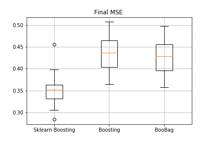
我们仍无法击败Sklearn的类似物，因为同样，我们没有考虑该方法中使用的许多参数。 但是，我们看到套袋会有所帮助。

让我们不要灰心，继续写XGBoost。

4. XGBoost

在继续阅读之前，强烈建议您先熟悉下一个视频 ，该视频很好地解释了这一理论。

回想一下在正常提升中我们最小化的错误：

$$

$$err（h）= \ sum_ {j = 1} ^ N L（\ sum_ {i = 1} ^ {T-1} a_ib_i（x_j）+ b_Ta_T（x_j））$$

XGBoost显式将正则化添加到此错误功能：

$$

$$err（h）= \ sum_ {j = 1} ^ NL（\ sum_ {i = 1} ^ {T-1} a_ib_i（x_j）+ b_Ta_T（x_j））+ \ sum_ {i = 1} ^ T \欧米茄（a_i）$$

如何考虑此功能？ 首先，我们借助二阶泰勒级数对其进行近似，其中新算法被认为是我们将沿其运动的增量，然后我们已经根据所具有的损失类型进行了绘制：

$$$f（x + \ delta x）\ thinapprox f（x）+ f（x）'\ delta x + 0.5 * f（x）''（\ delta x）^ 2$

有必要确定我们认为哪棵树不好，哪棵树好。

回想一下构建什么原理回归 $$$L_2$-正则化-回归之前的系数值越正常，越差，因此有必要使其尽可能小。

在XGBoost中，想法非常相似：如果树中叶子的值的范数之和很大，则对树进行罚款。 因此，树的复杂性介绍如下：

$$

$$\ omega（a）= \ gamma Z + 0.5 * \ sum_ {i = 1} ^ {Z} w_i ^ 2$$

$$$w$-叶子中的价值， $$$Z$-叶数。

视频中有转换公式，我们在这里不显示它们。 归结为以下事实：我们将选择一个新分区，以最大化收益：

$$

$$增益= \ frac {G_l ^ 2} {S_l ^ 2 + \ lambda} + \ frac {G_r ^ 2} {S_r ^ 2 + \ lambda}-\ frac {（G_l + G_r）^ 2} {S_l ^ 2 + S_r ^ 2 + \ lambda}-\ gamma$$

在这里 $$$\ gamma，\ lambda$是正则化的数值参数，并且 $$$G_i，S_i$-此分区的一阶和二阶导数的相应总和。

就是这样，理论非常简短，给出了链接，现在让我们讨论一下如果与MSE合作，衍生产品将是什么。 很简单：

$$$mse（y，预测）=（y-预测）^ 2 \\ \ nabla_ {预测} mse（y，预测）=预测-y \\ \ nabla_ {predict} ^ 2 mse（y，预测）= 1$

我们什么时候计算金额 $$$G_i，S_i$，只需添加到第一个 $$$预测-y$第二个就是数量。

 %%cython -a import numpy as np cimport numpy as np cdef class RegressionTreeGain: cdef public int max_depth cdef public np.float64_t gain cdef public np.float64_t lmd cdef public np.float64_t gmm cdef public int feature_idx cdef public int min_size cdef public np.float64_t feature_threshold cdef public np.float64_t value cpdef public RegressionTreeGain left cpdef public RegressionTreeGain right def __init__(self, int max_depth=3, np.float64_t lmd=1.0, np.float64_t gmm=0.1, min_size=5): self.max_depth = max_depth self.gmm = gmm self.lmd = lmd self.left = None self.right = None self.feature_idx = -1 self.feature_threshold = 0 self.value = -1e9 self.min_size = min_size return def fit(self, np.ndarray[np.float64_t, ndim=2] X, np.ndarray[np.float64_t, ndim=1] y): cpdef long N = X.shape[0] cpdef long N1 = X.shape[0] cpdef long N2 = 0 cpdef long idx = 0 cpdef long thres = 0 cpdef np.float64_t gl, gr, gn cpdef np.ndarray[long, ndim=1] idxs cpdef np.float64_t x = 0.0 cpdef np.float64_t best_gain = -self.gmm if self.value == -1e9: self.value = y.mean() base_error = ((y - self.value) ** 2).sum() error = base_error flag = 0 if self.max_depth <= 1: return dim_shape = X.shape[1] left_value = 0 right_value = 0 #    # -  -   mse, L = (y - pred)**2 # dL/dpred = pred - y,          - # dL^2/d^2pred = 1 - ,       for feat in range(dim_shape): idxs = np.argsort(X[:, feat]) gl,gr = y.sum(),0.0 N1, N2, thres = N, 0, 0 while thres < N - 1: N1 -= 1 N2 += 1 idx = idxs[thres] x = X[idx, feat] gl -= y[idx] gr += y[idx] #   gn = (gl**2) / (N1 + self.lmd) + (gr**2) / (N2 + self.lmd) gn -= ((gl + gr)**2) / (N1 + N2 + self.lmd) + self.gmm if thres < N - 1 and x == X[idxs[thres + 1], feat]: thres += 1 continue #     if (gn > best_gain) and (min(N1,N2) > self.min_size): flag = 1 best_gain = gn left_value = -gl / (N1 + self.lmd) right_value = -gr / (N2 + self.lmd) self.feature_idx = feat self.feature_threshold = x thres += 1 self.gain = best_gain if self.feature_idx == -1: return self.left = RegressionTreeGain(max_depth=self.max_depth - 1, gmm=self.gmm, lmd=self.lmd) self.left.value = left_value self.right = RegressionTreeGain(max_depth=self.max_depth - 1, gmm=self.gmm, lmd=self.lmd) self.right.value = right_value idxs_l = (X[:, self.feature_idx] > self.feature_threshold) idxs_r = (X[:, self.feature_idx] <= self.feature_threshold) self.left.fit(X[idxs_l, :], y[idxs_l]) self.right.fit(X[idxs_r, :], y[idxs_r]) #    if (self.left.left == None or self.right.left == None): if self.gain < 0.0: self.left = None self.right = None self.feature_idx = -1 def __predict(self, np.ndarray[np.float64_t, ndim=1] x): if self.feature_idx == -1: return self.value if x[self.feature_idx] > self.feature_threshold: return self.left.__predict(x) else: return self.right.__predict(x) def predict(self, np.ndarray[np.float64_t, ndim=2] X): y = np.zeros(X.shape[0]) for i in range(X.shape[0]): y[i] = self.__predict(X[i]) return y 

一个小小的澄清：为了使树木中的公式变得更漂亮，在加速时我们用减号训练目标。

我们稍微修改一下增强，使一些参数自适应。 例如，如果我们注意到损失已经开始达到平稳状态，则我们降低学习率并增加以下估计量的max_depth。 我们还将添加一个新的套袋-现在，我们将利用收益来增强树套袋：

 class Bagging(): def __init__(self, max_depth = 3, min_size=5, n_samples = 10): self.max_depth = max_depth self.min_size = min_size self.n_samples = n_samples self.subsample_size = None self.list_of_Carts = [RegressionTreeGain(max_depth=self.max_depth, min_size=self.min_size) for _ in range(self.n_samples)] def get_bootstrap_samples(self, data_train, y_train): indices = np.random.randint(0, len(data_train), (self.n_samples, self.subsample_size)) samples_train = data_train[indices] samples_y = y_train[indices] return samples_train, samples_y def fit(self, data_train, y_train): self.subsample_size = int(data_train.shape[0]) samples_train, samples_y = self.get_bootstrap_samples(data_train, y_train) for i in range(self.n_samples): self.list_of_Carts[i].fit(samples_train[i], samples_y[i].reshape(-1)) return self def predict(self, test_data): num_samples = test_data.shape[0] pred = [] for i in range(self.n_samples): pred.append(self.list_of_Carts[i].predict(test_data)) pred = np.array(pred).T return np.array([np.mean(pred[i]) for i in range(num_samples)]) 

 class GradientBoosting(): def __init__(self, n_estimators=100, learning_rate=0.2, max_depth=3, random_state=17, n_samples = 15, min_size = 5, base_tree='Bagging'): self.n_estimators = n_estimators self.max_depth = max_depth self.learning_rate = learning_rate self.initialization = lambda y: np.mean(y) * np.ones([y.shape[0]]) self.min_size = min_size self.loss_by_iter = [] self.trees_ = [] self.loss_by_iter_test = [] self.n_samples = n_samples self.base_tree = base_tree #  -       #   ,   lr   max_depth self.add_to_max_depth = 1 self.init_mse_board = 1.5 def fit(self, X, y): print (self.base_tree) self.X = X self.y = y b = self.initialization(y) prediction = b.copy() for t in tqdm_notebook(range(self.n_estimators)): if t == 0: resid = y else: resid = (y - prediction) if (mse(temp_resid,resid) < self.init_mse_board): self.init_mse_board /= 1.5 self.add_to_max_depth += 1 self.learning_rate /= 1.1 # print ('Alert!', t, self.add_to_max_depth) if self.base_tree == 'Bagging': tree = Bagging(max_depth=self.max_depth+self.add_to_max_depth, min_size = self.min_size) resid = -resid if self.base_tree == 'Tree': tree = RegressionTreeFastMse(max_depth=self.max_depth+self.add_to_max_depth, min_size = self.min_size) if self.base_tree == 'XGBoost': tree = RegressionTreeGain(max_depth=self.max_depth+self.add_to_max_depth, min_size = self.min_size) resid = -resid tree.fit(X, resid) b = tree.predict(X).reshape([X.shape[0]]) # print (b.shape) self.trees_.append(tree) prediction += self.learning_rate * b temp_resid = resid return self def predict(self, X): #   –          pred = np.ones([X.shape[0]]) * np.mean(self.y) #    for t in range(self.n_estimators): pred += self.learning_rate * self.trees_[t].predict(X).reshape([X.shape[0]]) return pred 

5.结果

按照传统，我们比较结果：

 data = datasets.fetch_california_housing() X = np.array(data.data) y = np.array(data.target) import matplotlib.pyplot as plt from sklearn.ensemble import GradientBoostingRegressor as GDBSklearn er_boosting_bagging = get_metrics(X,y,30,GradientBoosting(max_depth=3, n_estimators=150,base_tree='Bagging')) er_boosting_xgb = get_metrics(X,y,30,GradientBoosting(max_depth=3, n_estimators=150,base_tree='XGBoost')) er_sklearn_boosting = get_metrics(X,y,30,GDBSklearn(max_depth=3,n_estimators=150,learning_rate=0.2)) %matplotlib inline data = [er_sklearn_boosting, er_boosting_xgb, er_boosting_bagging] fig7, ax7 = plt.subplots() ax7.set_title('') ax7.boxplot(data, labels=['GdbSklearn', 'Xgboost', 'XGBooBag']) plt.grid() plt.show() 

图片如下：



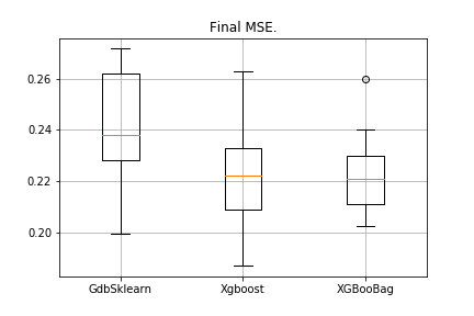
XGBoost的错误最少，但是XGBooBag的错误更拥挤，这绝对是更好的选择：算法更稳定。

仅此而已。 我真的希望两篇文章中介绍的材料是有用的，并且您可以自己学习一些新知识。 我特别感谢Dmitry提供了全面的反馈和源代码，感谢Anton提供了建议，并感谢Vladimir帮助完成了艰巨的任务。

一切成功！