引言
在Habr上发表了几篇文章[1,2,3],这些文章直接或间接地与此主题相关。 在这方面,大家一定会注意到标题为“手指上的数学:线性二次调节器”的出版物[1],该出版物通俗地解释了最佳LQR控制器的工作原理。
在研究了动态优化方法的实际应用之后,我想继续这个主题,但是已经在使用Python的一个具体示例中进行了探讨。 首先,简要介绍一下动态优化的术语和方法。
优化方法分为静态和动态。 控制对象在各种外部和内部因素的影响下处于连续运动的状态。 因此,对控制时间T给出控制结果的评估,这是一个动态优化任务。
使用动态优化的方法,解决了在一定时间内分配有限资源的问题,并将目标函数写为一个积分函数。
解决此类问题的数学仪器是变分方法:经典的变分演算,最大L.S.原理。 Pontryagin和动态编程R. Bellman。
在时间,频率和状态空间中执行控制系统的分析和综合。 状态空间中控制系统的分析和综合被引入课程中,但是,使用SQR控制器的培训材料中介绍的技术是为Matlab设计的,不包含分析的实际示例。
该出版物的目的是使用众所周知的使用Python编程语言优化电驱动器和飞机的控制系统的示例,考虑在状态空间中分析和综合线性控制系统的方法。
动态优化方法的数学依据
为了进行优化,使用了振幅(MO),对称(CO)和折衷最优(KO)的标准。
解决状态空间中的优化问题时,线性平稳系统由向量矩阵方程式给出:
dotx= fracdxdt=A cdotx+B cdotu;y=C cdotx, (1)
最小控制能耗和最大速度的集成标准由功能设置:
Jx= int infty0(xTQx+uTRu+2xTNu)dt rightarrowmin, (2)
Ju= int infty0(yTQy+uTRu+2yTNu)dt rightarrow分钟。 (3)
控制律u形式为对状态变量x或对输出变量y的线性反馈:
u= pmKx,u= pmKy这样的控制使二次质量标准(2),(3)最小化。 在关系式(1)÷(3)中,Q和R分别是尺寸为[n×n]和[m×m]的对称正定矩阵; K是尺寸为[m×n]的常数系数的矩阵,其值不受限制。 如果省略输入参数N,则将其视为零。
这个问题的解决方案在状态空间中称为线性积分二次优化(LQR-optimization)问题,由以下表达式确定:
u=R−1BTPx其中矩阵P必须满足Ricatti方程:
ATP+PA+PBR−1BTP+Q=0标准(2),(3)也是矛盾的,因为第一项的实现需要一个无限大功率的源,而对于第二项,则需要无限低功率的源。 可以用以下表达式解释:
Jx= int infty0xTQxdt ,
这是常态
Mod(x) 向量x,即 调节过程中其振荡的量度,因此,在瞬态中以较小的振荡获得较小的值,表达式为:
Ju= int infty0uTRudt是用于控制的能量的量度;是对系统能量成本的惩罚。
权重矩阵Q,R和N取决于相应坐标的约束。 如果这些矩阵的任何元素等于零,则对应的坐标没有限制。 在实践中,矩阵Q,R,N的值的选择是通过专家估计,试验,误差的方法进行的,并且取决于设计工程师的经验和知识。
为了解决这些问题,使用了以下MATLAB运算符:
\开始bmatrixR,S,E\结束bmatrix=lqr(A,B,Q,R,N) 和
\开始bmatrixR,S,E\结束bmatrix=lqry(Ps,Q,R,N) 通过状态向量x或输出向量y最小化函数(2),(3)。
管理对象模型
Ps=ss(A,B,C,D) 计算结果是关于状态变量x的最佳反馈矩阵K,Ricatti方程S的解以及闭环控制系统的特征值E = eiq(A-BK)。
功能组件:
Jx=x0TP1x0,Ju=x0TP2x0其中x0是初始条件的向量;
P1 和
P2 -作为Lyapunov矩阵方程的解的未知矩阵。 使用函数可以找到它们。
P1=lyap(NN,Q) 和
P2=lyap(NN,KTRK) ,
NN=(A+BK)T使用Python实现动态优化方法的功能
尽管Python控制系统库[4]具有以下功能:control.lqr,control.lyap,但只有在安装了slycot模块的情况下,才能使用control.lqr,这是一个问题[5]。 在任务上下文中使用lyap函数时,优化会导致control.exception.ControlArgument:Q必须是对称矩阵错误[6]。
因此,为了实现lqr()和lyap()函数,我使用了scipy.linalg:
from numpy import* from scipy.linalg import* def lqr(A,B,Q,R): S =matrix(solve_continuous_are(A, B, Q, R)) K = matrix(inv(R)*(BT*S)) E= eig(AB*K)[0] return K, S, E P1=solve_lyapunov(NN,Ct*Q*C)
顺便说一下,您不应该完全放弃控制,因为函数step(),pole(),ss(),tf(),feedback(),acker(),place()和其他函数都可以正常工作。
电驱动中LQR优化的示例
(示例摘自出版物[7])考虑一个线性二次控制器的合成,该控制器满足通过矩阵在状态空间中定义的控制对象的标准(2):
A=\开始bmatrix&−100&0&0&143.678&−16.667&−195.402&0&1.046&0 endbmatrix;B=\开始bmatrix230000\结尾bmatrix;C=\开始bmatrix1&0&00&1&00&0&1 endbmatrix;D=0
以下内容被视为状态变量:
x1 -转换器电压,V;
x2 -电动机电流,A;
x3 -角速度
c−1 。 这是具有HB的TP-DPT系统:发动机R nom = 30 kW; Unom = 220 V; Inom = 147 A ;;
\ωω 0 = 169
c−1 ;
\ωω 最大值= 187
c−1 ; 标称电阻力矩Mnom = 150 N * m; 起动电流的倍数= 2; 晶闸管转换器:Unom = 230 V; Uy = 10 B; Inom = 300安; 短时过电流倍数= 1.2。
解决问题时,我们接受矩阵Q对角线。 作为建模的结果,发现矩阵元素的最小值R = 84,并且
Q=[[0.01,0,0],[0,0.01,0],[0,0,0.01]] 在这种情况下,观察到发动机角速度的单调过渡过程(图1)。 在R = 840时
Q=[[0.01,0,0],[0,0.01,0],[0,0,0.01]] 瞬态过程(图2)符合MO的标准。 矩阵P1和P2的计算在x0 = [220 147 162]下进行。
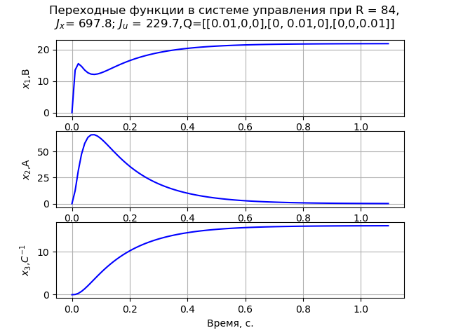 图 1个
图 1个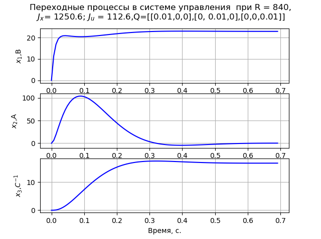 图 2
图 2通过适当选择矩阵R和Q,可以将电动机的启动电流减小到等于(2-2.5)In的可接受值(图3)。 例如,R = 840且
Q =([[[0.01,0,0],[0,0.88,0],[0,0,0.01]],其值为292 A,在这些条件下的过渡过程时间为1.57 s。

图3
在所有考虑的情况下,电压和电流的反馈均为负,速度的反馈为正,根据稳定性的要求,这是不希望的。 另外,综合系统对于任务是静态的,对于负载是静态的。 因此,我们考虑在状态空间中使用附加状态变量对PI控制器进行综合
x4 -积分器的传递系数。
我们以矩阵形式表示初始信息:
A=\开始bmatrix&−100&0&0&0&143.678&−16.667&−195.402&0&0&1.046&0&0&0&0&1&0 endbmatrix;B=\开始bmatrix2300000\结束bmatrix;C=眼睛(4));D=0在R = 100,q11 = q22 = q33 = 0.001和q44 = 200的情况下,获得了与MO标准相对应的任务瞬态。图4显示了状态变量瞬态,它通过任务和负载确认了系统的静态性。
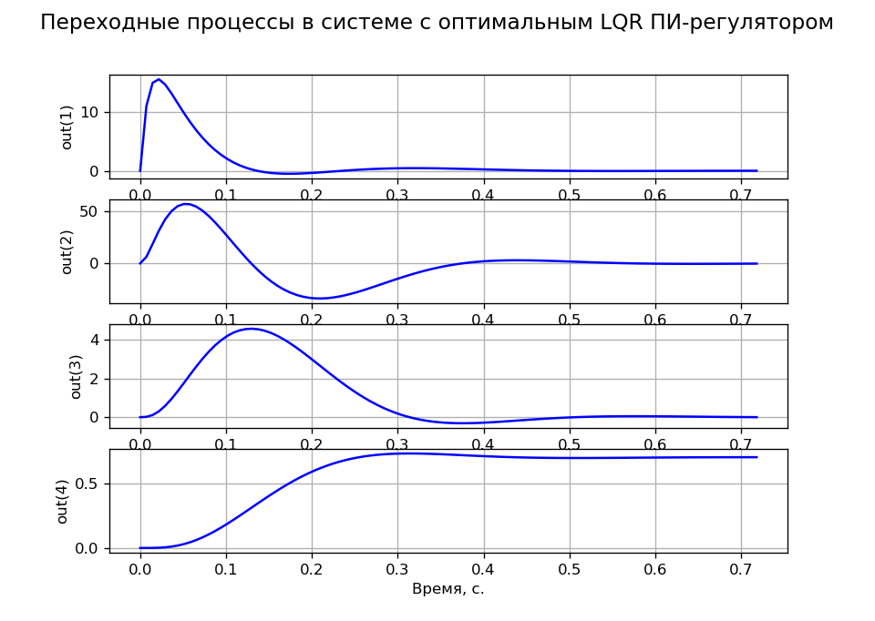 图 4
图 4为了确定矩阵K,Python控制系统库具有两个函数K = acker(A,B,s)和K = place(A,B,s),其中s是向量-闭环控制系统传递函数的期望极点所在的行。 第一条命令仅可用于u中n≤5且u中有一个输入的系统。 第二个没有这种限制,但是极点的多重性不应该超过矩阵B的秩。清单和(图5)中显示了使用acker()运算符的示例。
 图 5
图 5结论
考虑到新lqr()和lyap()函数的使用,该出版物中提出的LQR驱动优化的实现将使我们在研究控制理论的相应部分时放弃使用许可的MATLAB程序。
飞机(LA)中LQR优化的示例
(示例取自Astrom和Mruray的出版物,第5章[8],并由文章的作者最终完成,以取代lqr()函数并将术语引入公认的术语)理论部分,简要的理论,LQR优化已经在上面考虑过了,所以让我们继续进行代码分析并给出相应的注释:
所需的库和LQR控制器功能。 from scipy.linalg import*
初始条件和基本矩阵A,B,C,D模型。 xe = [0, 0, 0, 0, 0, 0];
我们建立与xy位置的逐步变化相对应的输入和输出。 向量xd和yd对应于系统中所需的稳态。 矩阵Cx和Cy是模型的相应输出。 为了描述系统的动力学,我们使用矢量矩阵方程组:
\左\ {\开始{矩阵} xdot = Ax + Bu => xdot =(A-BK)x + xd \\ u = -K(x-xd)\\ y = Cx \\ \结束{matrix} \对。
对于K \ cdot xd和K \ cdot xd作为输入向量,可以使用step()函数对闭环的动力学进行建模,其中:
xd = matrix([[1], [0], [0], [0], [0], [0]]); yd = matrix([[0], [1], [0], [0], [0], [0]]);
当前控件0.8.1库仅支持用于创建反馈控制器的SISO Matlab函数的一部分,因此,要从控制器读取数据,因此有必要为横向-x和垂直-y动态创建索引向量lat(),alt()。
lat = (0,2,3,5); alt = (1,4);
图形按顺序显示,每个任务一个。
figure(); title(" x y") plot(Tx.T, Yx.T, '-', Ty.T, Yy.T, '--'); plot([0, 10], [1, 1], 'k-'); axis([0, 10, -0.1, 1.4]); ylabel(' '); xlabel(''); legend(('x', 'y'), loc='lower right'); grid() show()
图表: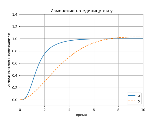 图表:
图表: 图表:
图表: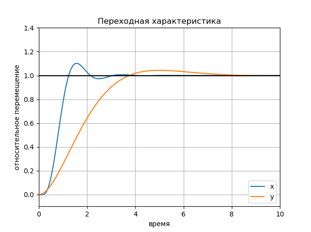 图表:
图表: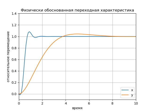
结论:
考虑到对新lqr()函数的使用,在出版物中介绍的飞机中LQR优化的实现允许我们在研究控制理论的相应部分时放弃使用许可程序MATLAB。
参考文献
1.
手指上的数学:线性二次控制器。2.
设计最优控制系统问题中的状态空间。3.
使用Python控制系统库设计自动控制系统。4.
Python控制系统库。5.
Python-无法将slycot模块导入spyder(RuntimeError和ImportError)。6.
Python控制系统库。7.
电动驱动器中最佳控制和lqr优化的标准。