神经常微分方程

微分方程描述了很大一部分过程，这可能是物理系统随时间的演变，患者的医疗状况，股票市场的基本特征等。从某种意义上说，观察只是状态不断变化的某种表现，有关这些过程的数据本质上是一致且连续的。

还有另一种串行数据类型，它是离散数据，例如NLP任务数据。此类数据中的状态离散地变化：从一个字符或单词到另一字符或单词。

现在，这两种类型的串行数据通常都由递归网络处理，尽管它们本质上不同并且似乎需要不同的方法。

上一届NIPS会议上发表了一篇非常有趣的文章，可以帮助解决此问题。作者提出了一种称为神经ODE的方法 。

在这里，我试图重现和总结本文的结果，以便使她的想法更容易理解。在我看来，这种新架构很可能会在数据科学家的标准工具中以及卷积和循环网络中找到一席之地。

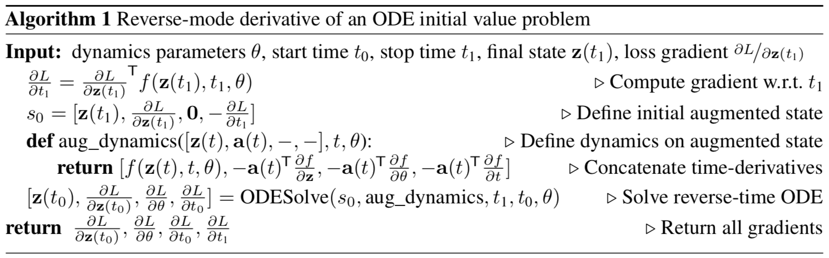
图 1：连续梯度反向传播需要及时解算出扩展的微分方程。

箭头表示通过观测值的梯度来调整向后传播的梯度。

原始文章中的插图。

问题陈述

假设有一个过程遵循某些未知的ODE，并且沿该过程的轨迹存在多个（嘈杂的）观察结果

$\ frac {dz} {dt} = f（z（t），t）\; （1）$

$\ {（z_0，t_0），（z_1，t_1），...，（z_M，t_M）\}-\文字{observations}$

如何找到一个近似值 $\ widehat {f}（z，t，\ theta）$ 扬声器功能 f（z，t）

？

首先，考虑一个简单的任务：在轨迹的开始和结尾只有2个观测值，（z_0，t_0），（z_1，t_1）

。

系统演进从状态开始 z_0，t_0

准时

可以使用ODE系统的任何演化方法使用一些参数化动力学函数。系统处于新状态后 $\ hat {z_1}，t_1$ ，与状态进行比较 z_1

并通过更改参数将它们之间的差异最小化 $\ theta$ 动力学功能。

或者，更正式地说，考虑最小化损失函数 $L（\帽子{z_1}）$ ：

$L（z（t_1））= L \大（\ int_ {t_0} ^ {t_1} f（z（t），t，\ theta）dt \ Big）= L \大（\文本{ODESolve}（z（ t_0），f，t_0，t_1，\ theta）\ big）\; （2）$

最小化

，您需要为其所有参数计算梯度： $z（t_0），t_0，t_1，\ theta$ 。为此，您首先需要确定如何

取决于每时每刻的状态（z [t））

：

$a（t）=-\ frac {\部分L} {\部分z（t）} \; （3）$

称为伴随状态，其动力学由另一个微分方程给出，可以将其视为复数函数微分（ 链规则 ）的连续模拟：

$\ frac {d a（t）} {d t} = -a（t）\ frac {\部分f（z（t），t，\ theta）} {\部分z} \; （4）$

该公式的输出可以在原始文章的附录中找到。

尽管原始文章同时使用行和列表示，但本文中的向量应被视为小写向量。

及时解决diffur（4），我们获得了对初始状态的依赖

：

$\ frac {\部分L} {\部分z（t_0）} = \ int_ {t_1} ^ {t_0} a（t）\ frac {\部分f（z（t），t，\ theta）} {\部分z} dt \; （5）$

计算相对于的梯度

和 $\ theta$ ，您可以简单地将其视为状态的一部分。这种情况称为增强。此状态的动态是从原始动态中轻松获得的：

$\ frac {d} {dt} \开始{bmatrix} z \\ \ theta \\ t \结束{bmatrix}（t）= f _ {\ text {aug}}（[z，\ theta，t]）：= \开始{bmatrix} f（[z，\ theta，t]）\\ 0 \\ 1 \结束{bmatrix} \; （6）$

然后将共轭状态扩展为该状态：

$a _ {\ text {aug}}：= \开始{bmatrix} a \\ a _ {\ theta} \\ a_t \ end {bmatrix}，a _ {\ theta}（t）：= \ frac {\部分L} { \\ partial \ theta（t）}，a_t（t）：= \ frac {\部分L} {\部分t（t）} \; （7）$

渐变增强动力学：

$\ frac {\部分f _ {\文本{aug}}} {\部分[z，\ theta，t]} = \开始{bmatrix} \ frac {\部分f} {\部分z}＆; \ frac {\部分f} {\部分\ theta}＆; \ frac {\部分f} {\部分t} \\ 0＆; 0＆; 0 \\ 0＆; 0＆; 0 \ end {bmatrix} \; （8）$

根据公式（4）得出的共轭增强态的微分方程为：

$\ frac {d a _ {\ text {aug}}} {dt} =-\开始{bmatrix} a \ frac {\部分f} {\部分z}＆; a \ frac {\部分f} {\部分\ theta}＆; a \ frac {\部分f} {\部分t} \结束{bmatrix} \; （9）$

及时解决此ODE会产生：

$\ frac {\部分L} {\部分z（t_0）} = \ int_ {t_1} ^ {t_0} a（t）\ frac {\部分f（z（t），t，\ theta）} {\部分z} dt \; （10）$

$\ frac {\部分L} {\部分\ theta} = \ int_ {t_1} ^ {t_0} a（t）\ frac {\部分f（z（t），t，\ theta）} {\部分\ theta } dt \; （11）$

$\ frac {\部分L} {\部分t_0} = \ int_ {t_1} ^ {t_0} a（t）\ frac {\部分f（z（t），t，\ theta）} {\部分t} dt \; （12）$

怎么了

$\ frac {\部分L} {\部分t_1} =-a（t）\ frac {\部分f（z（t），t，\ theta）} {\部分t} \; （13）$

在ODESolve ODE 解算器的所有输入参数中给出梯度。

所有梯度（10），（11），（12），（13）可以在一个ODESolve调用中与共轭增强态（9）的动力学一起计算。

原始文章中的插图。

上面的算法描述了连续观测的ODE解的梯度的反向传播。

在一个轨迹上进行多个观测的情况下，一切都以相同的方式计算，但是在观测的时刻，必须使用当前观测的梯度来调整分布梯度的倒数， 如图1所示。

实作

下面的代码是我对神经ODE的实现。我这样做纯粹是为了更好地了解正在发生的事情。但是，它与本文作者资源库中实现的内容非常接近。它包含您需要在一个地方理解的所有代码，并且注释也略多了。对于实际应用和实验，最好还是使用原始文章作者的实现。

import math import numpy as np from IPython.display import clear_output from tqdm import tqdm_notebook as tqdm import matplotlib as mpl import matplotlib.pyplot as plt %matplotlib inline import seaborn as sns sns.color_palette("bright") import matplotlib as mpl import matplotlib.cm as cm import torch from torch import Tensor from torch import nn from torch.nn import functional as F from torch.autograd import Variable use_cuda = torch.cuda.is_available()

首先，您需要实现ODE系统演化的任何方法。为简单起见，此处可以使用Euler方法，尽管任何显式或隐式方法都适用。

 def ode_solve(z0, t0, t1, f): """     -   """ h_max = 0.05 n_steps = math.ceil((abs(t1 - t0)/h_max).max().item()) h = (t1 - t0)/n_steps t = t0 z = z0 for i_step in range(n_steps): z = z + h * f(z, t) t = t + h return z

它还用一些有用的方法描述了参数化动力学函数的超类。

首先：您需要以向量的形式返回函数所依赖的所有参数。

其次：有必要计算增强动力。这种动力学取决于参数化函数在参数和输入数据方面的梯度。为了不必为每种新体系结构用每只手记录渐变，我们将使用torch.autograd.grad方法。

 class ODEF(nn.Module): def forward_with_grad(self, z, t, grad_outputs): """Compute f and a df/dz, a df/dp, a df/dt""" batch_size = z.shape[0] out = self.forward(z, t) a = grad_outputs adfdz, adfdt, *adfdp = torch.autograd.grad( (out,), (z, t) + tuple(self.parameters()), grad_outputs=(a), allow_unused=True, retain_graph=True ) #  grad       , #  expand   if adfdp is not None: adfdp = torch.cat([p_grad.flatten() for p_grad in adfdp]).unsqueeze(0) adfdp = adfdp.expand(batch_size, -1) / batch_size if adfdt is not None: adfdt = adfdt.expand(batch_size, 1) / batch_size return out, adfdz, adfdt, adfdp def flatten_parameters(self): p_shapes = [] flat_parameters = [] for p in self.parameters(): p_shapes.append(p.size()) flat_parameters.append(p.flatten()) return torch.cat(flat_parameters)

下面的代码描述了神经ODE的正向和反向传播。必须以torch.autograd.Function函数的形式将此代码与torch.nn.Module主代码分开，因为在后者中，您可以实现任意反向传播方法，这与模块不同。所以这只是拐杖。

此功能是整个神经ODE方法的基础。

 class ODEAdjoint(torch.autograd.Function): @staticmethod def forward(ctx, z0, t, flat_parameters, func): assert isinstance(func, ODEF) bs, *z_shape = z0.size() time_len = t.size(0) with torch.no_grad(): z = torch.zeros(time_len, bs, *z_shape).to(z0) z[0] = z0 for i_t in range(time_len - 1): z0 = ode_solve(z0, t[i_t], t[i_t+1], func) z[i_t+1] = z0 ctx.func = func ctx.save_for_backward(t, z.clone(), flat_parameters) return z @staticmethod def backward(ctx, dLdz): """ dLdz shape: time_len, batch_size, *z_shape """ func = ctx.func t, z, flat_parameters = ctx.saved_tensors time_len, bs, *z_shape = z.size() n_dim = np.prod(z_shape) n_params = flat_parameters.size(0) #   , #       def augmented_dynamics(aug_z_i, t_i): """   -     t_i -   : bs, 1 aug_z_i -   : bs, n_dim*2 + n_params + 1 """ #     z_i, a = aug_z_i[:, :n_dim], aug_z_i[:, n_dim:2*n_dim] # Unflatten z and a z_i = z_i.view(bs, *z_shape) a = a.view(bs, *z_shape) with torch.set_grad_enabled(True): t_i = t_i.detach().requires_grad_(True) z_i = z_i.detach().requires_grad_(True) faug = func.forward_with_grad(z_i, t_i, grad_outputs=a) func_eval, adfdz, adfdt, adfdp = faug adfdz = adfdz if adfdz is not None else torch.zeros(bs, *z_shape) adfdp = adfdp if adfdp is not None else torch.zeros(bs, n_params) adfdt = adfdt if adfdt is not None else torch.zeros(bs, 1) adfdz = adfdz.to(z_i) adfdp = adfdp.to(z_i) adfdt = adfdt.to(z_i) # Flatten f and adfdz func_eval = func_eval.view(bs, n_dim) adfdz = adfdz.view(bs, n_dim) return torch.cat((func_eval, -adfdz, -adfdp, -adfdt), dim=1) dLdz = dLdz.view(time_len, bs, n_dim) # flatten dLdz   with torch.no_grad(): ##      #    , #       adj_z = torch.zeros(bs, n_dim).to(dLdz) adj_p = torch.zeros(bs, n_params).to(dLdz) #    z  p,        adj_t = torch.zeros(time_len, bs, 1).to(dLdz) for i_t in range(time_len-1, 0, -1): z_i = z[i_t] t_i = t[i_t] f_i = func(z_i, t_i).view(bs, n_dim) #      dLdz_i = dLdz[i_t] dLdt_i = torch.bmm(torch.transpose(dLdz_i.unsqueeze(-1), 1, 2), f_i.unsqueeze(-1))[:, 0] #     adj_z += dLdz_i adj_t[i_t] = adj_t[i_t] - dLdt_i #      aug_z = torch.cat(( z_i.view(bs, n_dim), adj_z, torch.zeros(bs, n_params).to(z) adj_t[i_t]), dim=-1 ) #  ()      aug_ans = ode_solve(aug_z, t_i, t[i_t-1], augmented_dynamics) #       adj_z[:] = aug_ans[:, n_dim:2*n_dim] adj_p[:] += aug_ans[:, 2*n_dim:2*n_dim + n_params] adj_t[i_t-1] = aug_ans[:, 2*n_dim + n_params:] del aug_z, aug_ans ##         #    dLdz_0 = dLdz[0] dLdt_0 = torch.bmm(torch.transpose(dLdz_0.unsqueeze(-1), 1, 2), f_i.unsqueeze(-1))[:, 0] #  adj_z += dLdz_0 adj_t[0] = adj_t[0] - dLdt_0 return adj_z.view(bs, *z_shape), adj_t, adj_p, None

现在为方便起见，将此函数包装在nn.Module中 。

 class NeuralODE(nn.Module): def __init__(self, func): super(NeuralODE, self).__init__() assert isinstance(func, ODEF) self.func = func def forward(self, z0, t=Tensor([0., 1.]), return_whole_sequence=False): t = t.to(z0) z = ODEAdjoint.apply(z0, t, self.func.flatten_parameters(), self.func) if return_whole_sequence: return z else: return z[-1]

申请书

恢复真实动态功能（方法验证）

作为一项基本测试，现在让我们检查神经ODE是否可以使用观测数据恢复动力学的真实功能。

为此，我们首先确定ODE的动力学函数，根据其演化轨迹，然后尝试从随机参数化的动力学函数中恢复它。

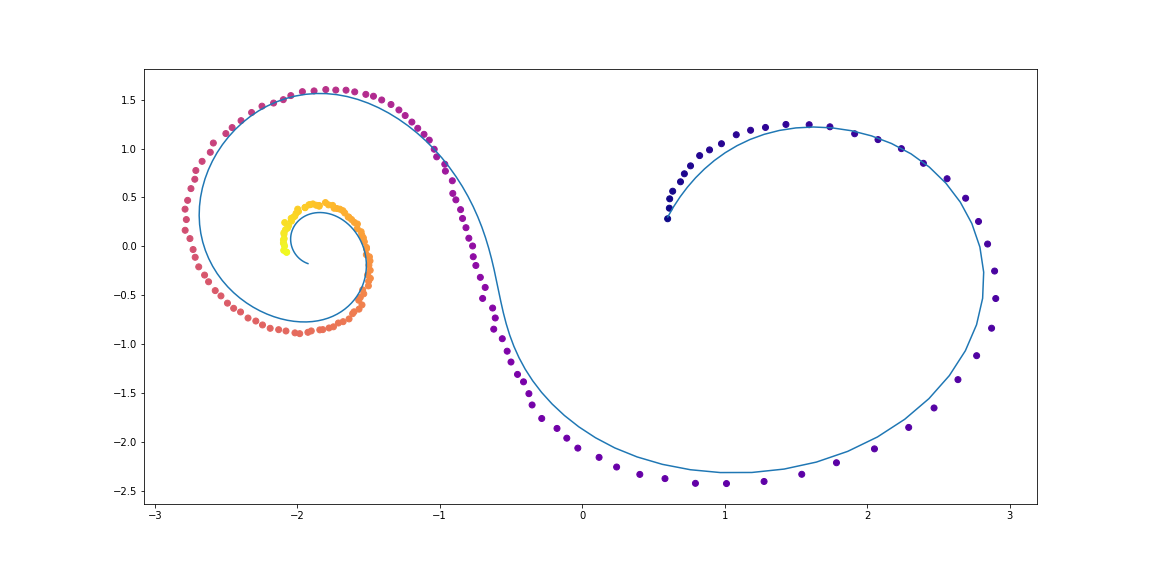
首先，让我们检查线性ODE的最简单情况。动力学的功能仅仅是矩阵的作用。

$\ frac {dz} {dt} = \开始{bmatrix} -0.1＆; -1.0 \\ 1.0＆; -0.1 \ end {bmatrix} z$

训练后的函数由随机矩阵参数化。

此外，还有一些更复杂的动态（没有gif，因为学习过程不是很漂亮：））
这里的学习功能是具有一个隐藏层的完全连接的网络。

代号

 class LinearODEF(ODEF): def __init__(self, W): super(LinearODEF, self).__init__() self.lin = nn.Linear(2, 2, bias=False) self.lin.weight = nn.Parameter(W) def forward(self, x, t): return self.lin(x)

动力学功能只是一个矩阵

 class SpiralFunctionExample(LinearODEF): def __init__(self): matrix = Tensor([[-0.1, -1.], [1., -0.1]]) super(SpiralFunctionExample, self).__init__(matrix)

随机参数化矩阵

 class RandomLinearODEF(LinearODEF): def __init__(self): super(RandomLinearODEF, self).__init__(torch.randn(2, 2)/2.)

动力学可实现更复杂的轨迹

 class TestODEF(ODEF): def __init__(self, A, B, x0): super(TestODEF, self).__init__() self.A = nn.Linear(2, 2, bias=False) self.A.weight = nn.Parameter(A) self.B = nn.Linear(2, 2, bias=False) self.B.weight = nn.Parameter(B) self.x0 = nn.Parameter(x0) def forward(self, x, t): xTx0 = torch.sum(x*self.x0, dim=1) dxdt = torch.sigmoid(xTx0) * self.A(x - self.x0) + torch.sigmoid(-xTx0) * self.B(x + self.x0) return dxdt

完全连接的网络形式的动态学习

 class NNODEF(ODEF): def __init__(self, in_dim, hid_dim, time_invariant=False): super(NNODEF, self).__init__() self.time_invariant = time_invariant if time_invariant: self.lin1 = nn.Linear(in_dim, hid_dim) else: self.lin1 = nn.Linear(in_dim+1, hid_dim) self.lin2 = nn.Linear(hid_dim, hid_dim) self.lin3 = nn.Linear(hid_dim, in_dim) self.elu = nn.ELU(inplace=True) def forward(self, x, t): if not self.time_invariant: x = torch.cat((x, t), dim=-1) h = self.elu(self.lin1(x)) h = self.elu(self.lin2(h)) out = self.lin3(h) return out def to_np(x): return x.detach().cpu().numpy() def plot_trajectories(obs=None, times=None, trajs=None, save=None, figsize=(16, 8)): plt.figure(figsize=figsize) if obs is not None: if times is None: times = [None] * len(obs) for o, t in zip(obs, times): o, t = to_np(o), to_np(t) for b_i in range(o.shape[1]): plt.scatter(o[:, b_i, 0], o[:, b_i, 1], c=t[:, b_i, 0], cmap=cm.plasma) if trajs is not None: for z in trajs: z = to_np(z) plt.plot(z[:, 0, 0], z[:, 0, 1], lw=1.5) if save is not None: plt.savefig(save) plt.show() def conduct_experiment(ode_true, ode_trained, n_steps, name, plot_freq=10): # Create data z0 = Variable(torch.Tensor([[0.6, 0.3]])) t_max = 6.29*5 n_points = 200 index_np = np.arange(0, n_points, 1, dtype=np.int) index_np = np.hstack([index_np[:, None]]) times_np = np.linspace(0, t_max, num=n_points) times_np = np.hstack([times_np[:, None]]) times = torch.from_numpy(times_np[:, :, None]).to(z0) obs = ode_true(z0, times, return_whole_sequence=True).detach() obs = obs + torch.randn_like(obs) * 0.01 # Get trajectory of random timespan min_delta_time = 1.0 max_delta_time = 5.0 max_points_num = 32 def create_batch(): t0 = np.random.uniform(0, t_max - max_delta_time) t1 = t0 + np.random.uniform(min_delta_time, max_delta_time) idx = sorted(np.random.permutation( index_np[(times_np > t0) & (times_np < t1)] )[:max_points_num]) obs_ = obs[idx] ts_ = times[idx] return obs_, ts_ # Train Neural ODE optimizer = torch.optim.Adam(ode_trained.parameters(), lr=0.01) for i in range(n_steps): obs_, ts_ = create_batch() z_ = ode_trained(obs_[0], ts_, return_whole_sequence=True) loss = F.mse_loss(z_, obs_.detach()) optimizer.zero_grad() loss.backward(retain_graph=True) optimizer.step() if i % plot_freq == 0: z_p = ode_trained(z0, times, return_whole_sequence=True) plot_trajectories(obs=[obs], times=[times], trajs=[z_p], save=f"assets/imgs/{name}/{i}.png") clear_output(wait=True) ode_true = NeuralODE(SpiralFunctionExample()) ode_trained = NeuralODE(RandomLinearODEF()) conduct_experiment(ode_true, ode_trained, 500, "linear") func = TestODEF(Tensor([[-0.1, -0.5], [0.5, -0.1]]), Tensor([[0.2, 1.], [-1, 0.2]]), Tensor([[-1., 0.]])) ode_true = NeuralODE(func) func = NNODEF(2, 16, time_invariant=True) ode_trained = NeuralODE(func) conduct_experiment(ode_true, ode_trained, 3000, "comp", plot_freq=30)

如您所见， Neural ODE在还原动力学方面做得很好。即，该概念作为整体起作用。
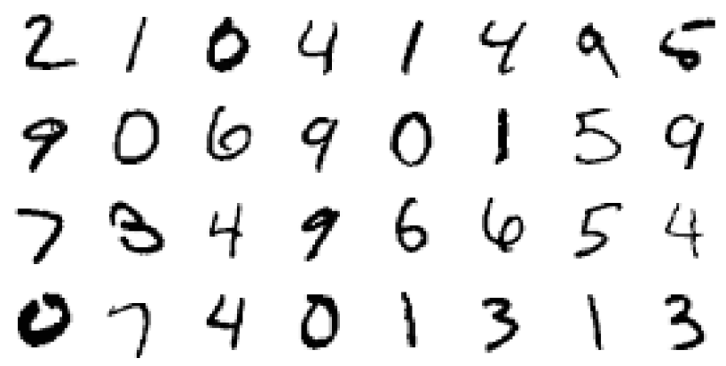
现在检查一个稍微复杂的问题（MNIST，哈哈）。

受ResNets启发的神经ODE

在ResNet'ax中，潜在状态根据公式更改

$h_ {t + 1} = h_ {t} + f（h_ {t}，\ theta_ {t}）$

在哪里 $t \ in \ {0 ... T \}$ 是块号和

这是块内各层学习到的功能。

在极限情况下，如果我们采用无限多的步长不断缩小的块，则与上面一样，我们将以ODE的形式获得隐藏层的连续动态。

$\ frac {dh（t）} {dt} = f（h（t），t，\ theta）$

从输入层开始

我们可以定义输出层

作为在时间T对该ODE的解决方案。

现在我们可以数 $\ theta$ 作为所有无穷小块之间的分布式（共享）参数。

在MNIST上验证神经ODE架构

在这一部分中，我们将测试神经ODE在更熟悉的体系结构中用作组件的功能。

特别是，我们将在MNIST分类器中将剩余块替换为神经ODE 。

代号

 def norm(dim): return nn.BatchNorm2d(dim) def conv3x3(in_feats, out_feats, stride=1): return nn.Conv2d(in_feats, out_feats, kernel_size=3, stride=stride, padding=1, bias=False) def add_time(in_tensor, t): bs, c, w, h = in_tensor.shape return torch.cat((in_tensor, t.expand(bs, 1, w, h)), dim=1) class ConvODEF(ODEF): def __init__(self, dim): super(ConvODEF, self).__init__() self.conv1 = conv3x3(dim + 1, dim) self.norm1 = norm(dim) self.conv2 = conv3x3(dim + 1, dim) self.norm2 = norm(dim) def forward(self, x, t): xt = add_time(x, t) h = self.norm1(torch.relu(self.conv1(xt))) ht = add_time(h, t) dxdt = self.norm2(torch.relu(self.conv2(ht))) return dxdt class ContinuousNeuralMNISTClassifier(nn.Module): def __init__(self, ode): super(ContinuousNeuralMNISTClassifier, self).__init__() self.downsampling = nn.Sequential( nn.Conv2d(1, 64, 3, 1), norm(64), nn.ReLU(inplace=True), nn.Conv2d(64, 64, 4, 2, 1), norm(64), nn.ReLU(inplace=True), nn.Conv2d(64, 64, 4, 2, 1), ) self.feature = ode self.norm = norm(64) self.avg_pool = nn.AdaptiveAvgPool2d((1, 1)) self.fc = nn.Linear(64, 10) def forward(self, x): x = self.downsampling(x) x = self.feature(x) x = self.norm(x) x = self.avg_pool(x) shape = torch.prod(torch.tensor(x.shape[1:])).item() x = x.view(-1, shape) out = self.fc(x) return out func = ConvODEF(64) ode = NeuralODE(func) model = ContinuousNeuralMNISTClassifier(ode) if use_cuda: model = model.cuda() import torchvision img_std = 0.3081 img_mean = 0.1307 batch_size = 32 train_loader = torch.utils.data.DataLoader( torchvision.datasets.MNIST("data/mnist", train=True, download=True, transform=torchvision.transforms.Compose([ torchvision.transforms.ToTensor(), torchvision.transforms.Normalize((img_mean,), (img_std,)) ]) ), batch_size=batch_size, shuffle=True ) test_loader = torch.utils.data.DataLoader( torchvision.datasets.MNIST("data/mnist", train=False, download=True, transform=torchvision.transforms.Compose([ torchvision.transforms.ToTensor(), torchvision.transforms.Normalize((img_mean,), (img_std,)) ]) ), batch_size=128, shuffle=True ) optimizer = torch.optim.Adam(model.parameters()) def train(epoch): num_items = 0 train_losses = [] model.train() criterion = nn.CrossEntropyLoss() print(f"Training Epoch {epoch}...") for batch_idx, (data, target) in tqdm(enumerate(train_loader), total=len(train_loader)): if use_cuda: data = data.cuda() target = target.cuda() optimizer.zero_grad() output = model(data) loss = criterion(output, target) loss.backward() optimizer.step() train_losses += [loss.item()] num_items += data.shape[0] print('Train loss: {:.5f}'.format(np.mean(train_losses))) return train_losses def test(): accuracy = 0.0 num_items = 0 model.eval() criterion = nn.CrossEntropyLoss() print(f"Testing...") with torch.no_grad(): for batch_idx, (data, target) in tqdm(enumerate(test_loader), total=len(test_loader)): if use_cuda: data = data.cuda() target = target.cuda() output = model(data) accuracy += torch.sum(torch.argmax(output, dim=1) == target).item() num_items += data.shape[0] accuracy = accuracy * 100 / num_items print("Test Accuracy: {:.3f}%".format(accuracy)) n_epochs = 5 test() train_losses = [] for epoch in range(1, n_epochs + 1): train_losses += train(epoch) test() import pandas as pd plt.figure(figsize=(9, 5)) history = pd.DataFrame({"loss": train_losses}) history["cum_data"] = history.index * batch_size history["smooth_loss"] = history.loss.ewm(halflife=10).mean() history.plot(x="cum_data", y="smooth_loss", figsize=(12, 5), title="train error")

 Testing... 100% 79/79 [00:01<00:00, 45.69it/s] Test Accuracy: 9.740% Training Epoch 1... 100% 1875/1875 [01:15<00:00, 24.69it/s] Train loss: 0.20137 Testing... 100% 79/79 [00:01<00:00, 46.64it/s] Test Accuracy: 98.680% Training Epoch 2... 100% 1875/1875 [01:17<00:00, 24.32it/s] Train loss: 0.05059 Testing... 100% 79/79 [00:01<00:00, 46.11it/s] Test Accuracy: 97.760% Training Epoch 3... 100% 1875/1875 [01:16<00:00, 24.63it/s] Train loss: 0.03808 Testing... 100% 79/79 [00:01<00:00, 45.65it/s] Test Accuracy: 99.000% Training Epoch 4... 100% 1875/1875 [01:17<00:00, 24.28it/s] Train loss: 0.02894 Testing... 100% 79/79 [00:01<00:00, 45.42it/s] Test Accuracy: 99.130% Training Epoch 5... 100% 1875/1875 [01:16<00:00, 24.67it/s] Train loss: 0.02424 Testing... 100% 79/79 [00:01<00:00, 45.89it/s] Test Accuracy: 99.170%

在短短的5个时代和6分钟的训练中进行了非常粗略的训练后，该模型的测试误差已经小于1％。可以说， 神经ODE 作为组件很好地集成到了更传统的网络中。

在他们的文章中，作者还将该分类器（ODE-Net）与常规的全连接网络，具有相似架构的ResNet和具有完全相同的架构进行了比较，其中梯度直接通过ODESolve中的操作传播（没有共轭梯度方法）（ RK-Net）。

原始文章中的插图。

根据他们的说法，具有与神经网络ODE相同数量的参数的1层全连接网络在测试中具有更高的误差，具有相同误差的ResNet具有更多的参数，而没有共轭梯度法的RK-Net则具有较高的误差。并且随着内存消耗线性增加（允许的误差越小， ODESolve必须采取的步骤越多，这随步骤数线性增加了内存消耗）。

作者在其实现中使用具有自适应步长的隐式Runge-Kutta方法，这与此处更简单的Euler方法不同。他们还研究了新架构的一些属性。

ODE-Net功能（NFE转发-直接传递中的功能计算数）
原始文章中的插图。

（a）改变数值误差的可接受水平会改变直接分布的步数。
（b）直接分配所花费的时间与函数的计算次数成正比。
（c）向后传播中函数的计算数量大约是直接传播的一半，这表明共轭梯度方法可能比直接通过ODESolve传播梯度更有效。
（d）随着ODE-Net的训练越来越多，它需要对函数进行越来越多的计算（步伐越来越小），可能会适应模型日益增加的复杂性。

时间序列建模的隐藏生成功能

即使路径位于未知的隐藏空间中，Neural ODE也适合处理连续的串行数据。

在本节中，我们将使用Neural ODE尝试并更改连续序列的生成，并了解学习到的隐藏空间。

作者还将这一点与递归网络生成的相似序列进行了比较。

这里的实验与authors存储库中的相应示例稍有不同，这里的轨迹更加多样化。

资料

训练数据由随机螺旋组成，其中一半是顺时针方向，第二个是逆时针方向。此外，从这些螺旋中采样随机子序列，由编码递归模型在相反的方向上进行处理，从而产生初始的隐藏状态，然后逐渐发展，在隐藏空间中形成轨迹。然后将此潜在路径映射到数据空间，并与采样的子序列进行比较。因此，模型学习生成类似于数据集的轨迹。

数据集螺旋的示例

VAE作为生成模型

通过抽样程序生成模型：

$z_ {t_0} \ sim \ mathcal {N}（0，我）$

$z_ {t_1}，z_ {t_2}，...，z_ {t_M} = \文本{ODESolve}（z_ {t_0}，f，\ theta_f，t_0，...，t_M）$

$x_ {t_i} \ sim p（x \ mid z_ {t_i}; \ theta_x）$

可以使用变分自动编码器方法进行训练。

通过时间序列的递归编码器以获取时间参数 $\ mu_ {z_ {t_0}}$ ， $\ sigma_ {z_ {t_0}}$ 后验分布，然后从中取样：

$z_ {t_0} \ sim q \左（z_ {t_0} \中间x_ {t_0}，...，x_ {t_M}; t_0，...，t_M; \ theta_q \右）= \数学{N} \左（z_ {t_0} \中\ mu_ {z_ {t_0}} \ sigma_ {z_ {t_0}} \右）$

获取隐藏的轨迹：

$z_ {t_1}，z_ {t_2}，...，z_ {t_N} = \文本{ODESolve}（z_ {t_0}，f，\ theta_f，t_0，...，t_N），\文本{where} \ frac {dz} {dt} = f（z，t; \ theta_f）$

使用另一个神经网络将隐藏的路径映射到数据中的路径： $\ hat {x_ {t_i}}（z_ {t_i}，t_i; \ theta_x）$
最大化对采样路径的有效性下限（ELBO）的评估：

$\ text {ELBO} \大约N \ Big（\ sum_ {i = 0} ^ {M} \ log p（x_ {t_i} \ mid z_ {t_i}（z_ {t_0}; \ theta_f）; \ theta_x）+ KL \左（q（z_ {t_0} \中间x_ {t_0}，...，x_ {t_M}; t_0，...，t_M; \ theta_q）\并行\数学{N}（0，I）\右）\大）$

在高斯后验分布的情况下 $p（x \ mid z_ {t_i}; \ theta_x）$ 和已知的噪音水平 $\ sigma_x$ ：

$\ text {ELBO} \大约-N \ Big（\ sum_ {i = 1} ^ {M} \ frac {（x_i-\ hat {x_i}）^ 2} {\ sigma_x ^ 2}-\ log \ sigma_ { z_ {t_0}} ^ 2 + \ mu_ {z_ {t_0}} ^ 2 + \ sigma_ {z_ {t_0}} ^ 2 \大）+ C$

隐藏的ODE模型的计算图可以表示如下

原始文章中的插图。

然后可以仅使用初始观测值测试该模型的内插路径。

代号

定义模型

 class RNNEncoder(nn.Module): def __init__(self, input_dim, hidden_dim, latent_dim): super(RNNEncoder, self).__init__() self.input_dim = input_dim self.hidden_dim = hidden_dim self.latent_dim = latent_dim self.rnn = nn.GRU(input_dim+1, hidden_dim) self.hid2lat = nn.Linear(hidden_dim, 2*latent_dim) def forward(self, x, t): # Concatenate time to input t = t.clone() t[1:] = t[:-1] - t[1:] t[0] = 0. xt = torch.cat((x, t), dim=-1) _, h0 = self.rnn(xt.flip((0,))) # Reversed # Compute latent dimension z0 = self.hid2lat(h0[0]) z0_mean = z0[:, :self.latent_dim] z0_log_var = z0[:, self.latent_dim:] return z0_mean, z0_log_var class NeuralODEDecoder(nn.Module): def __init__(self, output_dim, hidden_dim, latent_dim): super(NeuralODEDecoder, self).__init__() self.output_dim = output_dim self.hidden_dim = hidden_dim self.latent_dim = latent_dim func = NNODEF(latent_dim, hidden_dim, time_invariant=True) self.ode = NeuralODE(func) self.l2h = nn.Linear(latent_dim, hidden_dim) self.h2o = nn.Linear(hidden_dim, output_dim) def forward(self, z0, t): zs = self.ode(z0, t, return_whole_sequence=True) hs = self.l2h(zs) xs = self.h2o(hs) return xs class ODEVAE(nn.Module): def __init__(self, output_dim, hidden_dim, latent_dim): super(ODEVAE, self).__init__() self.output_dim = output_dim self.hidden_dim = hidden_dim self.latent_dim = latent_dim self.encoder = RNNEncoder(output_dim, hidden_dim, latent_dim) self.decoder = NeuralODEDecoder(output_dim, hidden_dim, latent_dim) def forward(self, x, t, MAP=False): z_mean, z_log_var = self.encoder(x, t) if MAP: z = z_mean else: z = z_mean + torch.randn_like(z_mean) * torch.exp(0.5 * z_log_var) x_p = self.decoder(z, t) return x_p, z, z_mean, z_log_var def generate_with_seed(self, seed_x, t): seed_t_len = seed_x.shape[0] z_mean, z_log_var = self.encoder(seed_x, t[:seed_t_len]) x_p = self.decoder(z_mean, t) return x_p

数据集生成

 t_max = 6.29*5 n_points = 200 noise_std = 0.02 num_spirals = 1000 index_np = np.arange(0, n_points, 1, dtype=np.int) index_np = np.hstack([index_np[:, None]]) times_np = np.linspace(0, t_max, num=n_points) times_np = np.hstack([times_np[:, None]] * num_spirals) times = torch.from_numpy(times_np[:, :, None]).to(torch.float32) # Generate random spirals parameters normal01 = torch.distributions.Normal(0, 1.0) x0 = Variable(normal01.sample((num_spirals, 2))) * 2.0 W11 = -0.1 * normal01.sample((num_spirals,)).abs() - 0.05 W22 = -0.1 * normal01.sample((num_spirals,)).abs() - 0.05 W21 = -1.0 * normal01.sample((num_spirals,)).abs() W12 = 1.0 * normal01.sample((num_spirals,)).abs() xs_list = [] for i in range(num_spirals): if i % 2 == 1: # Make it counter-clockwise W21, W12 = W12, W21 func = LinearODEF(Tensor([[W11[i], W12[i]], [W21[i], W22[i]]])) ode = NeuralODE(func) xs = ode(x0[i:i+1], times[:, i:i+1], return_whole_sequence=True) xs_list.append(xs) orig_trajs = torch.cat(xs_list, dim=1).detach() samp_trajs = orig_trajs + torch.randn_like(orig_trajs) * noise_std samp_ts = times fig, axes = plt.subplots(nrows=3, ncols=3, figsize=(15, 9)) axes = axes.flatten() for i, ax in enumerate(axes): ax.scatter(samp_trajs[:, i, 0], samp_trajs[:, i, 1], c=samp_ts[:, i, 0], cmap=cm.plasma) plt.show() import numpy.random as npr def gen_batch(batch_size, n_sample=100): n_batches = samp_trajs.shape[1] // batch_size time_len = samp_trajs.shape[0] n_sample = min(n_sample, time_len) for i in range(n_batches): if n_sample > 0: probs = [1. / (time_len - n_sample)] * (time_len - n_sample) t0_idx = npr.multinomial(1, probs) t0_idx = np.argmax(t0_idx) tM_idx = t0_idx + n_sample else: t0_idx = 0 tM_idx = time_len frm, to = batch_size*i, batch_size*(i+1) yield samp_trajs[t0_idx:tM_idx, frm:to], samp_ts[t0_idx:tM_idx, frm:to]

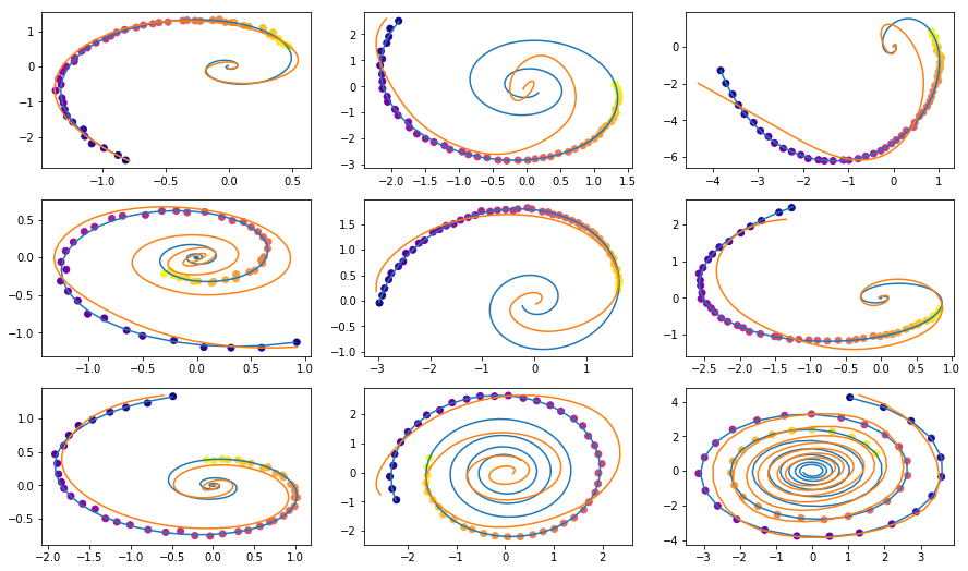
培训课程

 vae = ODEVAE(2, 64, 6) vae = vae.cuda() if use_cuda: vae = vae.cuda() optim = torch.optim.Adam(vae.parameters(), betas=(0.9, 0.999), lr=0.001) preload = False n_epochs = 20000 batch_size = 100 plot_traj_idx = 1 plot_traj = orig_trajs[:, plot_traj_idx:plot_traj_idx+1] plot_obs = samp_trajs[:, plot_traj_idx:plot_traj_idx+1] plot_ts = samp_ts[:, plot_traj_idx:plot_traj_idx+1] if use_cuda: plot_traj = plot_traj.cuda() plot_obs = plot_obs.cuda() plot_ts = plot_ts.cuda() if preload: vae.load_state_dict(torch.load("models/vae_spirals.sd")) for epoch_idx in range(n_epochs): losses = [] train_iter = gen_batch(batch_size) for x, t in train_iter: optim.zero_grad() if use_cuda: x, t = x.cuda(), t.cuda() max_len = np.random.choice([30, 50, 100]) permutation = np.random.permutation(t.shape[0]) np.random.shuffle(permutation) permutation = np.sort(permutation[:max_len]) x, t = x[permutation], t[permutation] x_p, z, z_mean, z_log_var = vae(x, t) z_var = torch.exp(z_log_var) kl_loss = -0.5 * torch.sum(1 + z_log_var - z_mean**2 - z_var, -1) loss = 0.5 * ((x-x_p)**2).sum(-1).sum(0) / noise_std**2 + kl_loss loss = torch.mean(loss) loss /= max_len loss.backward() optim.step() losses.append(loss.item()) print(f"Epoch {epoch_idx}") frm, to, to_seed = 0, 200, 50 seed_trajs = samp_trajs[frm:to_seed] ts = samp_ts[frm:to] if use_cuda: seed_trajs = seed_trajs.cuda() ts = ts.cuda() samp_trajs_p = to_np(vae.generate_with_seed(seed_trajs, ts)) fig, axes = plt.subplots(nrows=3, ncols=3, figsize=(15, 9)) axes = axes.flatten() for i, ax in enumerate(axes): ax.scatter(to_np(seed_trajs[:, i, 0]), to_np(seed_trajs[:, i, 1]), c=to_np(ts[frm:to_seed, i, 0]), cmap=cm.plasma) ax.plot(to_np(orig_trajs[frm:to, i, 0]), to_np(orig_trajs[frm:to, i, 1])) ax.plot(samp_trajs_p[:, i, 0], samp_trajs_p[:, i, 1]) plt.show() print(np.mean(losses), np.median(losses)) clear_output(wait=True) spiral_0_idx = 3 spiral_1_idx = 6 homotopy_p = Tensor(np.linspace(0., 1., 10)[:, None]) vae = vae if use_cuda: homotopy_p = homotopy_p.cuda() vae = vae.cuda() spiral_0 = orig_trajs[:, spiral_0_idx:spiral_0_idx+1, :] spiral_1 = orig_trajs[:, spiral_1_idx:spiral_1_idx+1, :] ts_0 = samp_ts[:, spiral_0_idx:spiral_0_idx+1, :] ts_1 = samp_ts[:, spiral_1_idx:spiral_1_idx+1, :] if use_cuda: spiral_0, ts_0 = spiral_0.cuda(), ts_0.cuda() spiral_1, ts_1 = spiral_1.cuda(), ts_1.cuda() z_cw, _ = vae.encoder(spiral_0, ts_0) z_cc, _ = vae.encoder(spiral_1, ts_1) homotopy_z = z_cw * (1 - homotopy_p) + z_cc * homotopy_p t = torch.from_numpy(np.linspace(0, 6*np.pi, 200)) t = t[:, None].expand(200, 10)[:, :, None].cuda() t = t.cuda() if use_cuda else t hom_gen_trajs = vae.decoder(homotopy_z, t) fig, axes = plt.subplots(nrows=2, ncols=5, figsize=(15, 5)) axes = axes.flatten() for i, ax in enumerate(axes): ax.plot(to_np(hom_gen_trajs[:, i, 0]), to_np(hom_gen_trajs[:, i, 1])) plt.show() torch.save(vae.state_dict(), "models/vae_spirals.sd")