哈Ha!
去年秋天,在Kaggle举行了一场比赛,为手绘Quick Draw Doodle Recognition图片进行了分类,其中包括由
Artem Klevtsov ,
Philip Upravitelev和
Andrey Ogurtsov组成的R-schiks团队。 我们不会详细描述比赛,这已经在
最近的出版物中做了。
这次农场没有奖牌,但是获得了很多宝贵的经验,所以我想向社区介绍Kagl和日常工作中最有趣和最有用的一些东西。 涉及的主题包括:没有
OpenCV的艰苦生活,JSON解析(这些示例
显示了使用
Rcpp将C ++代码集成到R中的脚本或程序包中),脚本的参数化和最终解决方案的dockerization。
存储库中提供了消息中适合启动的所有代码。
内容:
- 有效地将数据从CSV加载到MonetDB数据库
- 批量准备
- 用于从数据库中卸载批次的迭代器
- 模型架构选择
- 脚本参数化
- 对接脚本
- 在Google Cloud中使用多个GPU
- 而不是结论
1.有效地将数据从CSV加载到MonetDB数据库
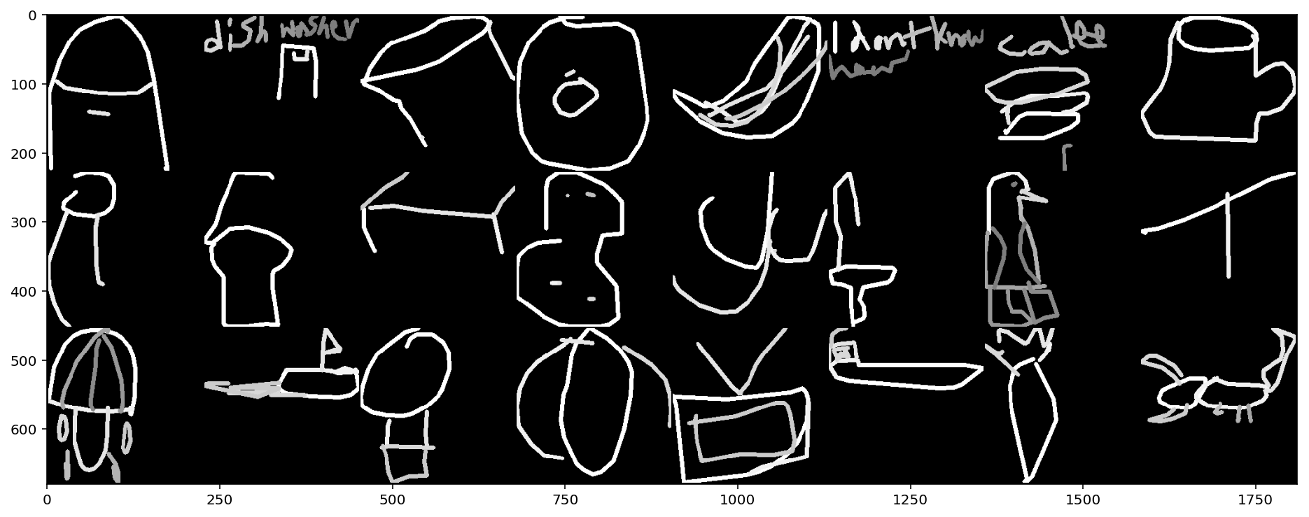
本次比赛中的数据不是以现成图片的形式提供,而是以340个CSV文件(每个类一个文件)的形式提供,其中包含带有点坐标的JSON。 将这些点与线连接起来,我们得到的最终图像尺寸为256x256像素。 另外,对于每条记录,都会给标签加上图片,以便在收集数据集时使用的分类器正确识别图片,作者的居住国的两个字母的代码,唯一的标识符,时间戳和与文件名匹配的类名。 简化版本的源数据在存档中的重量为7.4 GB,解压缩后的重量约为20 GB,解压缩后的完整数据需要240 GB。 组织者保证两个版本都复制相同的图纸,即完整版本是多余的。 无论如何,立即将5000万张图像存储在图形文件或数组中被认为是无利可图的,我们决定将train_simplified.zip存档中的所有CSV文件合并到数据库中,并随后为每批动态生成合适大小的图像。
选择成熟的MonetDB作为DBMS,即采用MonetDBLite包形式的R实现。 该软件包包括数据库服务器的嵌入式版本,允许您直接从R会话中提起服务器并在其中使用它。 创建数据库并连接到数据库是通过以下命令执行的:
con <- DBI::dbConnect(drv = MonetDBLite::MonetDBLite(), Sys.getenv("DBDIR"))
我们将需要创建两个表:一个表用于所有数据,另一个表用于有关已下载文件的服务信息(如果出现问题,将很有用,并且在下载多个文件后必须恢复该过程):
建立表格 if (!DBI::dbExistsTable(con, "doodles")) { DBI::dbCreateTable( con = con, name = "doodles", fields = c( "countrycode" = "char(2)", "drawing" = "text", "key_id" = "bigint", "recognized" = "bool", "timestamp" = "timestamp", "word" = "text" ) ) } if (!DBI::dbExistsTable(con, "upload_log")) { DBI::dbCreateTable( con = con, name = "upload_log", fields = c( "id" = "serial", "file_name" = "text UNIQUE", "uploaded" = "bool DEFAULT false" ) ) }
将数据加载到数据库的最快方法是使用SQL直接复制CSV文件-命令COPY OFFSET 2 INTO tablename FROM path USING DELIMITERS ',','\\n','\"' NULL AS '' BEST EFFORT using COPY OFFSET 2 INTO tablename FROM path USING DELIMITERS ',','\\n','\"' NULL AS '' BEST EFFORT ,其中tablename是表和path的名称是文件的路径。后来,发现了另一种提高速度的方法:用LOCKED BEST EFFORT替换BEST EFFORT 。当使用存档时,事实证明R中的内置unzip实现无法与存档中的许多文件一起正常工作,因此我们使用系统unzip (使用getOption("unzip")参数)。
写入数据库的功能 #' @title #' #' @description #' CSV- ZIP- #' #' @param con ( `MonetDBEmbeddedConnection`). #' @param tablename . #' @oaram zipfile ZIP-. #' @oaram filename ZIP-. #' @param preprocess , . #' `data` ( `data.table`). #' #' @return `TRUE`. #' upload_file <- function(con, tablename, zipfile, filename, preprocess = NULL) { # checkmate::assert_class(con, "MonetDBEmbeddedConnection") checkmate::assert_string(tablename) checkmate::assert_string(filename) checkmate::assert_true(DBI::dbExistsTable(con, tablename)) checkmate::assert_file_exists(zipfile, access = "r", extension = "zip") checkmate::assert_function(preprocess, args = c("data"), null.ok = TRUE) # path <- file.path(tempdir(), filename) unzip(zipfile, files = filename, exdir = tempdir(), junkpaths = TRUE, unzip = getOption("unzip")) on.exit(unlink(file.path(path))) # if (!is.null(preprocess)) { .data <- data.table::fread(file = path) .data <- preprocess(data = .data) data.table::fwrite(x = .data, file = path, append = FALSE) rm(.data) } # CSV sql <- sprintf( "COPY OFFSET 2 INTO %s FROM '%s' USING DELIMITERS ',','\\n','\"' NULL AS '' BEST EFFORT", tablename, path ) # DBI::dbExecute(con, sql) # DBI::dbExecute(con, sprintf("INSERT INTO upload_log(file_name, uploaded) VALUES('%s', true)", filename)) return(invisible(TRUE)) }
如果需要在写入数据库之前转换表,则足以传递将数据转换为preprocess参数的函数。
用于将数据顺序加载到数据库中的代码:
将数据写入数据库 # files <- unzip(zipfile, list = TRUE)$Name # , to_skip <- DBI::dbGetQuery(con, "SELECT file_name FROM upload_log")[[1L]] files <- setdiff(files, to_skip) if (length(files) > 0L) { # tictoc::tic() # pb <- txtProgressBar(min = 0L, max = length(files), style = 3) for (i in seq_along(files)) { upload_file(con = con, tablename = "doodles", zipfile = zipfile, filename = files[i]) setTxtProgressBar(pb, i) } close(pb) # tictoc::toc() } # 526.141 sec elapsed - SSD->SSD # 558.879 sec elapsed - USB->SSD
数据加载时间可能会因所使用驱动器的速度特性而异。 在我们的情况下,在同一SSD内或从USB闪存驱动器(源文件)到SSD(数据库)进行读写不到10分钟。
创建带有整数类标签的列和带有行号的索引列( ORDERED INDEX )会花费几秒钟的时间,这将用于选择创建批处理时的情况:
创建其他列和索引 message("Generate lables") invisible(DBI::dbExecute(con, "ALTER TABLE doodles ADD label_int int")) invisible(DBI::dbExecute(con, "UPDATE doodles SET label_int = dense_rank() OVER (ORDER BY word) - 1")) message("Generate row numbers") invisible(DBI::dbExecute(con, "ALTER TABLE doodles ADD id serial")) invisible(DBI::dbExecute(con, "CREATE ORDERED INDEX doodles_id_ord_idx ON doodles(id)"))
为了解决“即时”创建批处理的问题,我们需要实现从doodles表中提取随机字符串的最大速度。 为此,我们使用了3个技巧。 第一个是减小存储观察ID的类型的尺寸。 在原始数据集中,需要使用bigint类型来存储ID,但是观察次数可以使它们的标识符(与序列号相同)适合int类型。 搜索速度更快。 第二个技巧是使用ORDERED INDEX这个决定是凭经验做出的,对所有可用选项进行了排序。 第三是使用参数化查询。 该方法的本质是执行一次PREPARE命令,然后在创建相同类型的查询堆时使用准备好的表达式,但实际上,与简单的SELECT相比,其收益在于统计错误。
填充数据的过程不超过450 MB的RAM。 也就是说,所描述的方法允许您在几乎任何预算的硬件(包括一些单板计算机)上旋转重达数十GB的数据集,这非常酷。
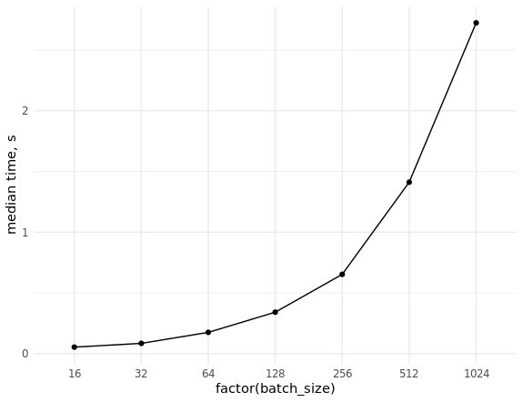
在对不同大小的批次进行采样时,仍然需要测量(随机)数据的提取率并评估缩放比例:
基准数据库 library(ggplot2) set.seed(0) # con <- DBI::dbConnect(MonetDBLite::MonetDBLite(), Sys.getenv("DBDIR")) # prep_sql <- function(batch_size) { sql <- sprintf("PREPARE SELECT id FROM doodles WHERE id IN (%s)", paste(rep("?", batch_size), collapse = ",")) res <- DBI::dbSendQuery(con, sql) return(res) } # fetch_data <- function(rs, batch_size) { ids <- sample(seq_len(n), batch_size) res <- DBI::dbFetch(DBI::dbBind(rs, as.list(ids))) return(res) } # res_bench <- bench::press( batch_size = 2^(4:10), { rs <- prep_sql(batch_size) bench::mark( fetch_data(rs, batch_size), min_iterations = 50L ) } ) # cols <- c("batch_size", "min", "median", "max", "itr/sec", "total_time", "n_itr") res_bench[, cols] # batch_size min median max `itr/sec` total_time n_itr # <dbl> <bch:tm> <bch:tm> <bch:tm> <dbl> <bch:tm> <int> # 1 16 23.6ms 54.02ms 93.43ms 18.8 2.6s 49 # 2 32 38ms 84.83ms 151.55ms 11.4 4.29s 49 # 3 64 63.3ms 175.54ms 248.94ms 5.85 8.54s 50 # 4 128 83.2ms 341.52ms 496.24ms 3.00 16.69s 50 # 5 256 232.8ms 653.21ms 847.44ms 1.58 31.66s 50 # 6 512 784.6ms 1.41s 1.98s 0.740 1.1m 49 # 7 1024 681.7ms 2.72s 4.06s 0.377 2.16m 49 ggplot(res_bench, aes(x = factor(batch_size), y = median, group = 1)) + geom_point() + geom_line() + ylab("median time, s") + theme_minimal() DBI::dbDisconnect(con, shutdown = TRUE)
2.批次的准备
批生产的整个过程包括以下步骤:
- 解析包含线向量和点坐标的多个JSON。
- 通过所需大小的图像中的点的坐标绘制彩色线(例如256x256或128x128)。
- 将生成的图像转换为张量。
在Python内核之间的竞争框架下,主要通过OpenCV解决了该问题。 R上最简单,最明显的类似物之一如下所示:
在R上实现JSON至张量转换 r_process_json_str <- function(json, line.width = 3, color = TRUE, scale = 1) { # JSON coords <- jsonlite::fromJSON(json, simplifyMatrix = FALSE) tmp <- tempfile() # on.exit(unlink(tmp)) png(filename = tmp, width = 256 * scale, height = 256 * scale, pointsize = 1) # plot.new() # plot.window(xlim = c(256 * scale, 0), ylim = c(256 * scale, 0)) # cols <- if (color) rainbow(length(coords)) else "#000000" for (i in seq_along(coords)) { lines(x = coords[[i]][[1]] * scale, y = coords[[i]][[2]] * scale, col = cols[i], lwd = line.width) } dev.off() # 3- res <- png::readPNG(tmp) return(res) } r_process_json_vector <- function(x, ...) { res <- lapply(x, r_process_json_str, ...) # 3- 4- res <- do.call(abind::abind, c(res, along = 0)) return(res) }
使用标准R工具执行绘图,并将其保存到RAM中存储的临时PNG中(在Linux中,临时R目录位于RAM中安装的/tmp中)。 然后,以3维数组的形式读取此文件,其数字范围为0到1。这很重要,因为更常见的BMP将被读取为带有十六进制颜色代码的原始数组。
测试结果:
zip_file <- file.path("data", "train_simplified.zip") csv_file <- "cat.csv" unzip(zip_file, files = csv_file, exdir = tempdir(), junkpaths = TRUE, unzip = getOption("unzip")) tmp_data <- data.table::fread(file.path(tempdir(), csv_file), sep = ",", select = "drawing", nrows = 10000) arr <- r_process_json_str(tmp_data[4, drawing]) dim(arr) # [1] 256 256 3 plot(magick::image_read(arr))

批次本身将形成如下:
res <- r_process_json_vector(tmp_data[1:4, drawing], scale = 0.5) str(res) # num [1:4, 1:128, 1:128, 1:3] 1 1 1 1 1 1 1 1 1 1 ... # - attr(*, "dimnames")=List of 4 # ..$ : NULL # ..$ : NULL # ..$ : NULL # ..$ : NULL
在我们看来,这种实现并不是最佳选择,因为大批量的生产花费了很长时间,并且我们决定使用功能强大的OpenCV库来利用同事的经验。 当时,没有用于R的现成软件包(甚至现在都没有),因此使用Rcpp将其集成到R代码中, 从而编写了C ++中所需功能的最小实现。
为了解决该问题,使用了以下软件包和库:
- OpenCV用于成像和线条绘制。 我们使用了预安装的系统库和头文件,以及动态链接。
- xtensor用于处理多维数组和张量。 我们使用了包含在同名R-package中的头文件。 该库使您可以按行主顺序和列主顺序使用多维数组。
- ndjson用于解析JSON。 当项目中可用时,该库会自动在xtensor中使用。
- RcppThread用于组织来自JSON的向量的多线程处理。 使用了此软件包提供的头文件。 该程序包的内置中断机制与更流行的RcppParallel有所不同。
值得注意的是, xtensor只是一个发现:除了具有广泛的功能和高性能之外, xtensor的开发人员还具有很强的响应能力,并及时详细地回答了出现的问题。 在他们的帮助下,可以将OpenCV矩阵转换为张量张量,以及将3维图像张量组合为正确尺寸的4维张量(实际上是批处理)的方法。
Rcpp,xtensor和RcppThread的学习资料 为了使用系统文件编译文件并与系统中安装的库进行动态链接,我们使用了Rcpp软件包中实现的插件机制。 为了自动查找路径和标志,我们使用了流行的linux实用程序pkg-config 。
实施Rcpp插件以使用OpenCV库 Rcpp::registerPlugin("opencv", function() { # pkg_config_name <- c("opencv", "opencv4") # pkg-config pkg_config_bin <- Sys.which("pkg-config") # checkmate::assert_file_exists(pkg_config_bin, access = "x") # OpenCV pkg-config check <- sapply(pkg_config_name, function(pkg) system(paste(pkg_config_bin, pkg))) if (all(check != 0)) { stop("OpenCV config for the pkg-config not found", call. = FALSE) } pkg_config_name <- pkg_config_name[check == 0] list(env = list( PKG_CXXFLAGS = system(paste(pkg_config_bin, "--cflags", pkg_config_name), intern = TRUE), PKG_LIBS = system(paste(pkg_config_bin, "--libs", pkg_config_name), intern = TRUE) )) })
作为插件的结果,在编译期间,将替换以下值:
Rcpp:::.plugins$opencv()$env # $PKG_CXXFLAGS # [1] "-I/usr/include/opencv" # # $PKG_LIBS # [1] "-lopencv_shape -lopencv_stitching -lopencv_superres -lopencv_videostab -lopencv_aruco -lopencv_bgsegm -lopencv_bioinspired -lopencv_ccalib -lopencv_datasets -lopencv_dpm -lopencv_face -lopencv_freetype -lopencv_fuzzy -lopencv_hdf -lopencv_line_descriptor -lopencv_optflow -lopencv_video -lopencv_plot -lopencv_reg -lopencv_saliency -lopencv_stereo -lopencv_structured_light -lopencv_phase_unwrapping -lopencv_rgbd -lopencv_viz -lopencv_surface_matching -lopencv_text -lopencv_ximgproc -lopencv_calib3d -lopencv_features2d -lopencv_flann -lopencv_xobjdetect -lopencv_objdetect -lopencv_ml -lopencv_xphoto -lopencv_highgui -lopencv_videoio -lopencv_imgcodecs -lopencv_photo -lopencv_imgproc -lopencv_core"
在剧透器下给出了用于实现JSON解析和创建批处理以传输到模型的代码。 首先,添加本地项目目录以搜索头文件(ndjson所需):
Sys.setenv("PKG_CXXFLAGS" = paste0("-I", normalizePath(file.path("src"))))
在C ++中实现JSON到张量转换 // [[Rcpp::plugins(cpp14)]] // [[Rcpp::plugins(opencv)]] // [[Rcpp::depends(xtensor)]] // [[Rcpp::depends(RcppThread)]] #include <xtensor/xjson.hpp> #include <xtensor/xadapt.hpp> #include <xtensor/xview.hpp> #include <xtensor-r/rtensor.hpp> #include <opencv2/core/core.hpp> #include <opencv2/highgui/highgui.hpp> #include <opencv2/imgproc/imgproc.hpp> #include <Rcpp.h> #include <RcppThread.h> // using RcppThread::parallelFor; using json = nlohmann::json; using points = xt::xtensor<double,2>; // JSON using strokes = std::vector<points>; // JSON using xtensor3d = xt::xtensor<double, 3>; // using xtensor4d = xt::xtensor<double, 4>; // using rtensor3d = xt::rtensor<double, 3>; // R using rtensor4d = xt::rtensor<double, 4>; // R // // const static int SIZE = 256; // // . https://en.wikipedia.org/wiki/Pixel_connectivity#2-dimensional const static int LINE_TYPE = cv::LINE_4; // const static int LINE_WIDTH = 3; // // https://docs.opencv.org/3.1.0/da/d54/group__imgproc__transform.html#ga5bb5a1fea74ea38e1a5445ca803ff121 const static int RESIZE_TYPE = cv::INTER_LINEAR; // OpenCV- template <typename T, int NCH, typename XT=xt::xtensor<T,3,xt::layout_type::column_major>> XT to_xt(const cv::Mat_<cv::Vec<T, NCH>>& src) { // std::vector<int> shape = {src.rows, src.cols, NCH}; // size_t size = src.total() * NCH; // cv::Mat xt::xtensor XT res = xt::adapt((T*) src.data, size, xt::no_ownership(), shape); return res; } // JSON strokes parse_json(const std::string& x) { auto j = json::parse(x); // if (!j.is_array()) { throw std::runtime_error("'x' must be JSON array."); } strokes res; res.reserve(j.size()); for (const auto& a: j) { // 2- if (!a.is_array() || a.size() != 2) { throw std::runtime_error("'x' must include only 2d arrays."); } // auto p = a.get<points>(); res.push_back(p); } return res; } // // HSV cv::Mat ocv_draw_lines(const strokes& x, bool color = true) { // auto stype = color ? CV_8UC3 : CV_8UC1; // auto dtype = color ? CV_32FC3 : CV_32FC1; auto bg = color ? cv::Scalar(0, 0, 255) : cv::Scalar(255); auto col = color ? cv::Scalar(0, 255, 220) : cv::Scalar(0); cv::Mat img = cv::Mat(SIZE, SIZE, stype, bg); // size_t n = x.size(); for (const auto& s: x) { // size_t n_points = s.shape()[1]; for (size_t i = 0; i < n_points - 1; ++i) { // cv::Point from(s(0, i), s(1, i)); // cv::Point to(s(0, i + 1), s(1, i + 1)); // cv::line(img, from, to, col, LINE_WIDTH, LINE_TYPE); } if (color) { // col[0] += 180 / n; } } if (color) { // RGB cv::cvtColor(img, img, cv::COLOR_HSV2RGB); } // float32 [0, 1] img.convertTo(img, dtype, 1 / 255.0); return img; } // JSON xtensor3d process(const std::string& x, double scale = 1.0, bool color = true) { auto p = parse_json(x); auto img = ocv_draw_lines(p, color); if (scale != 1) { cv::Mat out; cv::resize(img, out, cv::Size(), scale, scale, RESIZE_TYPE); cv::swap(img, out); out.release(); } xtensor3d arr = color ? to_xt<double,3>(img) : to_xt<double,1>(img); return arr; } // [[Rcpp::export]] rtensor3d cpp_process_json_str(const std::string& x, double scale = 1.0, bool color = true) { xtensor3d res = process(x, scale, color); return res; } // [[Rcpp::export]] rtensor4d cpp_process_json_vector(const std::vector<std::string>& x, double scale = 1.0, bool color = false) { size_t n = x.size(); size_t dim = floor(SIZE * scale); size_t channels = color ? 3 : 1; xtensor4d res({n, dim, dim, channels}); parallelFor(0, n, [&x, &res, scale, color](int i) { xtensor3d tmp = process(x[i], scale, color); auto view = xt::view(res, i, xt::all(), xt::all(), xt::all()); view = tmp; }); return res; }
该代码应放在src/cv_xt.cpp并使用命令Rcpp::sourceCpp(file = "src/cv_xt.cpp", env = .GlobalEnv) ; 您还需要从存储库中 nlohmann/json.hpp 才能正常工作 。 该代码分为几个功能:
to_xt用于将图像矩阵( cv::Mat )转换为张量xt::xtensor的模板函数;parse_json函数解析一个JSON字符串,提取点的坐标,将它们打包成一个向量;ocv_draw_lines从接收到的点向量ocv_draw_lines多色线;process -结合了上述功能,还增加了缩放结果图像的能力;cpp_process_json_str process函数的包装,将结果导出到R对象(多维数组);cpp_process_json_vector - cpp_process_json_str函数的包装,它使您可以在多线程模式下处理字符串向量。
要绘制多色线,使用HSV颜色模型,然后转换为RGB。 测试结果:
arr <- cpp_process_json_str(tmp_data[4, drawing]) dim(arr) # [1] 256 256 3 plot(magick::image_read(arr))

R和C ++中实现速度的比较 res_bench <- bench::mark( r_process_json_str(tmp_data[4, drawing], scale = 0.5), cpp_process_json_str(tmp_data[4, drawing], scale = 0.5), check = FALSE, min_iterations = 100 ) # cols <- c("expression", "min", "median", "max", "itr/sec", "total_time", "n_itr") res_bench[, cols] # expression min median max `itr/sec` total_time n_itr # <chr> <bch:tm> <bch:tm> <bch:tm> <dbl> <bch:tm> <int> # 1 r_process_json_str 3.49ms 3.55ms 4.47ms 273. 490ms 134 # 2 cpp_process_json_str 1.94ms 2.02ms 5.32ms 489. 497ms 243 library(ggplot2) # res_bench <- bench::press( batch_size = 2^(4:10), { .data <- tmp_data[sample(seq_len(.N), batch_size), drawing] bench::mark( r_process_json_vector(.data, scale = 0.5), cpp_process_json_vector(.data, scale = 0.5), min_iterations = 50, check = FALSE ) } ) res_bench[, cols] # expression batch_size min median max `itr/sec` total_time n_itr # <chr> <dbl> <bch:tm> <bch:tm> <bch:tm> <dbl> <bch:tm> <int> # 1 r 16 50.61ms 53.34ms 54.82ms 19.1 471.13ms 9 # 2 cpp 16 4.46ms 5.39ms 7.78ms 192. 474.09ms 91 # 3 r 32 105.7ms 109.74ms 212.26ms 7.69 6.5s 50 # 4 cpp 32 7.76ms 10.97ms 15.23ms 95.6 522.78ms 50 # 5 r 64 211.41ms 226.18ms 332.65ms 3.85 12.99s 50 # 6 cpp 64 25.09ms 27.34ms 32.04ms 36.0 1.39s 50 # 7 r 128 534.5ms 627.92ms 659.08ms 1.61 31.03s 50 # 8 cpp 128 56.37ms 58.46ms 66.03ms 16.9 2.95s 50 # 9 r 256 1.15s 1.18s 1.29s 0.851 58.78s 50 # 10 cpp 256 114.97ms 117.39ms 130.09ms 8.45 5.92s 50 # 11 r 512 2.09s 2.15s 2.32s 0.463 1.8m 50 # 12 cpp 512 230.81ms 235.6ms 261.99ms 4.18 11.97s 50 # 13 r 1024 4s 4.22s 4.4s 0.238 3.5m 50 # 14 cpp 1024 410.48ms 431.43ms 462.44ms 2.33 21.45s 50 ggplot(res_bench, aes(x = factor(batch_size), y = median, group = expression, color = expression)) + geom_point() + geom_line() + ylab("median time, s") + theme_minimal() + scale_color_discrete(name = "", labels = c("cpp", "r")) + theme(legend.position = "bottom")
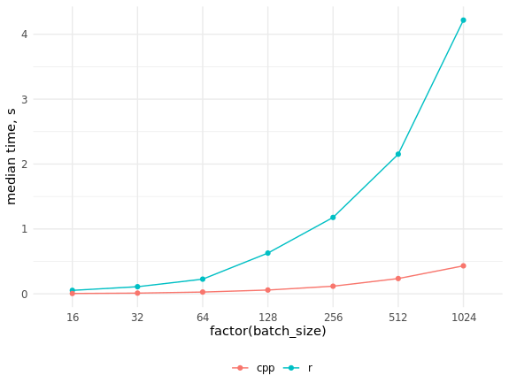
如您所见,速度的提高非常重要,并且不可能通过并行化R代码来赶上C ++代码。
3.用于从数据库中卸载批处理的迭代器
R作为一种用于处理位于RAM中的数据的语言而享有盛名,而Python的主要特色是迭代数据处理,这使得实现核外计算(使用外部存储器进行的计算)变得容易又容易。 在所描述问题的背景下,与我们有关的经典方法是深度计算神经网络,它是通过梯度下降方法训练的,其中每一步的梯度都由一小部分观测值或小批量进行近似。
用Python编写的深度学习框架具有特殊的类,这些类基于数据实现迭代器:表格,文件夹中的图片,二进制格式等。您可以使用现成的选项或为特定任务编写自己的选项。 在R中,我们可以使用具有相同名称的包充分利用Keras Python库及其各种后端,而该包又可以在网状包的顶部使用。 后者值得单独写一篇大文章; 它不仅允许您从R运行Python代码,而且还提供了R-和Python会话之间的对象传输,从而自动执行所有必要的类型转换。
由于使用了MonetDBLite,我们摆脱了将所有数据存储在RAM中的需要,所有的“神经网络”工作将由原始Python代码完成,我们只需要根据数据编写一个迭代器,因为R或Python中都没有针对这种情况的准备。 : ( R ). R numpy-, keras .
:
train_generator <- function(db_connection = con, samples_index, num_classes = 340, batch_size = 32, scale = 1, color = FALSE, imagenet_preproc = FALSE) { # checkmate::assert_class(con, "DBIConnection") checkmate::assert_integerish(samples_index) checkmate::assert_count(num_classes) checkmate::assert_count(batch_size) checkmate::assert_number(scale, lower = 0.001, upper = 5) checkmate::assert_flag(color) checkmate::assert_flag(imagenet_preproc) # , dt <- data.table::data.table(id = sample(samples_index)) # dt[, batch := (.I - 1L) %/% batch_size + 1L] # dt <- dt[, if (.N == batch_size) .SD, keyby = batch] # i <- 1 # max_i <- dt[, max(batch)] # sql <- sprintf( "PREPARE SELECT drawing, label_int FROM doodles WHERE id IN (%s)", paste(rep("?", batch_size), collapse = ",") ) res <- DBI::dbSendQuery(con, sql) # keras::to_categorical to_categorical <- function(x, num) { n <- length(x) m <- numeric(n * num) m[x * n + seq_len(n)] <- 1 dim(m) <- c(n, num) return(m) } # function() { # if (i > max_i) { dt[, id := sample(id)] data.table::setkey(dt, batch) # i <<- 1 max_i <<- dt[, max(batch)] } # ID batch_ind <- dt[batch == i, id] # batch <- DBI::dbFetch(DBI::dbBind(res, as.list(batch_ind)), n = -1) # i <<- i + 1 # JSON batch_x <- cpp_process_json_vector(batch$drawing, scale = scale, color = color) if (imagenet_preproc) { # c [0, 1] [-1, 1] batch_x <- (batch_x - 0.5) * 2 } batch_y <- to_categorical(batch$label_int, num_classes) result <- list(batch_x, batch_y) return(result) } }
, , , , ( scale = 1 256256 , scale = 0.5 — 128128 ), ( color = FALSE , color = TRUE ) , imagenet-. , [0, 1] [-1, 1], keras .
, data.table samples_index , , SQL- . keras::to_categorical() . , , steps_per_epoch keras::fit_generator() , if (i > max_i) .
, , JSON- ( cpp_process_json_vector() , C++) , . one-hot , , . data.table — "" data.table - R.
Core i5 :
library(Rcpp) library(keras) library(ggplot2) source("utils/rcpp.R") source("utils/keras_iterator.R") con <- DBI::dbConnect(drv = MonetDBLite::MonetDBLite(), Sys.getenv("DBDIR")) ind <- seq_len(DBI::dbGetQuery(con, "SELECT count(*) FROM doodles")[[1L]]) num_classes <- DBI::dbGetQuery(con, "SELECT max(label_int) + 1 FROM doodles")[[1L]] # train_ind <- sample(ind, floor(length(ind) * 0.995)) # val_ind <- ind[-train_ind] rm(ind) # scale <- 0.5 # res_bench <- bench::press( batch_size = 2^(4:10), { it1 <- train_generator( db_connection = con, samples_index = train_ind, num_classes = num_classes, batch_size = batch_size, scale = scale ) bench::mark( it1(), min_iterations = 50L ) } ) # cols <- c("batch_size", "min", "median", "max", "itr/sec", "total_time", "n_itr") res_bench[, cols] # batch_size min median max `itr/sec` total_time n_itr # <dbl> <bch:tm> <bch:tm> <bch:tm> <dbl> <bch:tm> <int> # 1 16 25ms 64.36ms 92.2ms 15.9 3.09s 49 # 2 32 48.4ms 118.13ms 197.24ms 8.17 5.88s 48 # 3 64 69.3ms 117.93ms 181.14ms 8.57 5.83s 50 # 4 128 157.2ms 240.74ms 503.87ms 3.85 12.71s 49 # 5 256 359.3ms 613.52ms 988.73ms 1.54 30.5s 47 # 6 512 884.7ms 1.53s 2.07s 0.674 1.11m 45 # 7 1024 2.7s 3.83s 5.47s 0.261 2.81m 44 ggplot(res_bench, aes(x = factor(batch_size), y = median, group = 1)) + geom_point() + geom_line() + ylab("median time, s") + theme_minimal() DBI::dbDisconnect(con, shutdown = TRUE)

, ( 32 ). /dev/shm , . , /etc/fstab , tmpfs /dev/shm tmpfs defaults,size=25g 0 0 . , df -h .
, :
test_generator <- function(dt, batch_size = 32, scale = 1, color = FALSE, imagenet_preproc = FALSE) { # checkmate::assert_data_table(dt) checkmate::assert_count(batch_size) checkmate::assert_number(scale, lower = 0.001, upper = 5) checkmate::assert_flag(color) checkmate::assert_flag(imagenet_preproc) # dt[, batch := (.I - 1L) %/% batch_size + 1L] data.table::setkey(dt, batch) i <- 1 max_i <- dt[, max(batch)] # function() { batch_x <- cpp_process_json_vector(dt[batch == i, drawing], scale = scale, color = color) if (imagenet_preproc) { # c [0, 1] [-1, 1] batch_x <- (batch_x - 0.5) * 2 } result <- list(batch_x) i <<- i + 1 return(result) } }
4.
mobilenet v1 , . keras , , R. : (batch, height, width, 3) , . Python , , ( , keras- ):
mobilenet v1 library(keras) top_3_categorical_accuracy <- custom_metric( name = "top_3_categorical_accuracy", metric_fn = function(y_true, y_pred) { metric_top_k_categorical_accuracy(y_true, y_pred, k = 3) } ) layer_sep_conv_bn <- function(object, filters, alpha = 1, depth_multiplier = 1, strides = c(2, 2)) { # NB! depth_multiplier != resolution multiplier # https://github.com/keras-team/keras/issues/10349 layer_depthwise_conv_2d( object = object, kernel_size = c(3, 3), strides = strides, padding = "same", depth_multiplier = depth_multiplier ) %>% layer_batch_normalization() %>% layer_activation_relu() %>% layer_conv_2d( filters = filters * alpha, kernel_size = c(1, 1), strides = c(1, 1) ) %>% layer_batch_normalization() %>% layer_activation_relu() } get_mobilenet_v1 <- function(input_shape = c(224, 224, 1), num_classes = 340, alpha = 1, depth_multiplier = 1, optimizer = optimizer_adam(lr = 0.002), loss = "categorical_crossentropy", metrics = c("categorical_crossentropy", top_3_categorical_accuracy)) { inputs <- layer_input(shape = input_shape) outputs <- inputs %>% layer_conv_2d(filters = 32, kernel_size = c(3, 3), strides = c(2, 2), padding = "same") %>% layer_batch_normalization() %>% layer_activation_relu() %>% layer_sep_conv_bn(filters = 64, strides = c(1, 1)) %>% layer_sep_conv_bn(filters = 128, strides = c(2, 2)) %>% layer_sep_conv_bn(filters = 128, strides = c(1, 1)) %>% layer_sep_conv_bn(filters = 256, strides = c(2, 2)) %>% layer_sep_conv_bn(filters = 256, strides = c(1, 1)) %>% layer_sep_conv_bn(filters = 512, strides = c(2, 2)) %>% layer_sep_conv_bn(filters = 512, strides = c(1, 1)) %>% layer_sep_conv_bn(filters = 512, strides = c(1, 1)) %>% layer_sep_conv_bn(filters = 512, strides = c(1, 1)) %>% layer_sep_conv_bn(filters = 512, strides = c(1, 1)) %>% layer_sep_conv_bn(filters = 512, strides = c(1, 1)) %>% layer_sep_conv_bn(filters = 1024, strides = c(2, 2)) %>% layer_sep_conv_bn(filters = 1024, strides = c(1, 1)) %>% layer_global_average_pooling_2d() %>% layer_dense(units = num_classes) %>% layer_activation_softmax() model <- keras_model( inputs = inputs, outputs = outputs ) model %>% compile( optimizer = optimizer, loss = loss, metrics = metrics ) return(model) }
. , , , . , imagenet-. , . get_config() ( base_model_conf$layers — R- ), from_config() :
base_model_conf <- get_config(base_model) base_model_conf$layers[[1]]$config$batch_input_shape[[4]] <- 1L base_model <- from_config(base_model_conf)
keras imagenet- :
get_model <- function(name = "mobilenet_v2", input_shape = NULL, weights = "imagenet", pooling = "avg", num_classes = NULL, optimizer = keras::optimizer_adam(lr = 0.002), loss = "categorical_crossentropy", metrics = NULL, color = TRUE, compile = FALSE) { # checkmate::assert_string(name) checkmate::assert_integerish(input_shape, lower = 1, upper = 256, len = 3) checkmate::assert_count(num_classes) checkmate::assert_flag(color) checkmate::assert_flag(compile) # keras model_fun <- get0(paste0("application_", name), envir = asNamespace("keras")) # if (is.null(model_fun)) { stop("Model ", shQuote(name), " not found.", call. = FALSE) } base_model <- model_fun( input_shape = input_shape, include_top = FALSE, weights = weights, pooling = pooling ) # , if (!color) { base_model_conf <- keras::get_config(base_model) base_model_conf$layers[[1]]$config$batch_input_shape[[4]] <- 1L base_model <- keras::from_config(base_model_conf) } predictions <- keras::get_layer(base_model, "global_average_pooling2d_1")$output predictions <- keras::layer_dense(predictions, units = num_classes, activation = "softmax") model <- keras::keras_model( inputs = base_model$input, outputs = predictions ) if (compile) { keras::compile( object = model, optimizer = optimizer, loss = loss, metrics = metrics ) } return(model) }
. : get_weights() R- , ( - ), set_weights() . , , .
mobilenet 1 2, resnet34. , SE-ResNeXt. , , ( ).
5.
, docopt :
doc <- ' Usage: train_nn.R --help train_nn.R --list-models train_nn.R [options] Options: -h --help Show this message. -l --list-models List available models. -m --model=<model> Neural network model name [default: mobilenet_v2]. -b --batch-size=<size> Batch size [default: 32]. -s --scale-factor=<ratio> Scale factor [default: 0.5]. -c --color Use color lines [default: FALSE]. -d --db-dir=<path> Path to database directory [default: Sys.getenv("db_dir")]. -r --validate-ratio=<ratio> Validate sample ratio [default: 0.995]. -n --n-gpu=<number> Number of GPUs [default: 1]. ' args <- docopt::docopt(doc)
docopt http://docopt.org/ R. Rscript bin/train_nn.R -m resnet50 -c -d /home/andrey/doodle_db ./bin/train_nn.R -m resnet50 -c -d /home/andrey/doodle_db , train_nn.R ( resnet50 128128 , /home/andrey/doodle_db ). , . , mobilenet_v2 keras R - R- — , .
RStudio ( tfruns ). , RStudio.
6.
. R- .
« », . , NVIDIA, CUDA+cuDNN — , tensorflow/tensorflow:1.12.0-gpu , R-.
- :
Dockerfile FROM tensorflow/tensorflow:1.12.0-gpu MAINTAINER Artem Klevtsov <aaklevtsov@gmail.com> SHELL ["/bin/bash", "-c"] ARG LOCALE="en_US.UTF-8" ARG APT_PKG="libopencv-dev r-base r-base-dev littler" ARG R_BIN_PKG="futile.logger checkmate data.table rcpp rapidjsonr dbi keras jsonlite curl digest remotes" ARG R_SRC_PKG="xtensor RcppThread docopt MonetDBLite" ARG PY_PIP_PKG="keras" ARG DIRS="/db /app /app/data /app/models /app/logs" RUN source /etc/os-release && \ echo "deb https://cloud.r-project.org/bin/linux/ubuntu ${UBUNTU_CODENAME}-cran35/" > /etc/apt/sources.list.d/cran35.list && \ apt-key adv --keyserver keyserver.ubuntu.com --recv-keys E084DAB9 && \ add-apt-repository -y ppa:marutter/c2d4u3.5 && \ add-apt-repository -y ppa:timsc/opencv-3.4 && \ apt-get update && \ apt-get install -y locales && \ locale-gen ${LOCALE} && \ apt-get install -y --no-install-recommends ${APT_PKG} && \ ln -s /usr/lib/R/site-library/littler/examples/install.r /usr/local/bin/install.r && \ ln -s /usr/lib/R/site-library/littler/examples/install2.r /usr/local/bin/install2.r && \ ln -s /usr/lib/R/site-library/littler/examples/installGithub.r /usr/local/bin/installGithub.r && \ echo 'options(Ncpus = parallel::detectCores())' >> /etc/R/Rprofile.site && \ echo 'options(repos = c(CRAN = "https://cloud.r-project.org"))' >> /etc/R/Rprofile.site && \ apt-get install -y $(printf "r-cran-%s " ${R_BIN_PKG}) && \ install.r ${R_SRC_PKG} && \ pip install ${PY_PIP_PKG} && \ mkdir -p ${DIRS} && \ chmod 777 ${DIRS} && \ rm -rf /tmp/downloaded_packages/ /tmp/*.rds && \ rm -rf /var/lib/apt/lists/* COPY utils /app/utils COPY src /app/src COPY tests /app/tests COPY bin/*.R /app/ ENV DBDIR="/db" ENV CUDA_HOME="/usr/local/cuda" ENV PATH="/app:${PATH}" WORKDIR /app VOLUME /db VOLUME /app CMD bash
; . /bin/bash /etc/os-release . .
-, . , , , :
#!/bin/sh DBDIR=${PWD}/db LOGSDIR=${PWD}/logs MODELDIR=${PWD}/models DATADIR=${PWD}/data ARGS="--runtime=nvidia --rm -v ${DBDIR}:/db -v ${LOGSDIR}:/app/logs -v ${MODELDIR}:/app/models -v ${DATADIR}:/app/data" if [ -z "$1" ]; then CMD="Rscript /app/train_nn.R" elif [ "$1" = "bash" ]; then ARGS="${ARGS} -ti" else CMD="Rscript /app/train_nn.R $@" fi docker run ${ARGS} doodles-tf ${CMD}
- , train_nn.R ; — "bash", . : CMD="Rscript /app/train_nn.R $@" .
, , , .
7. GPU Google Cloud
(. , @Leigh.plt ODS-). , 1 GPU GPU . GoogleCloud ( ) - , $300. 4V100 SSD , . , . K80. — SSD c, dev/shm .
, GPU. CPU , :
with(tensorflow::tf$device("/cpu:0"), { model_cpu <- get_model( name = model_name, input_shape = input_shape, weights = weights, metrics =(top_3_categorical_accuracy, compile = FALSE ) })
( ) GPU, :
model <- keras::multi_gpu_model(model_cpu, gpus = n_gpu) keras::compile( object = model, optimizer = keras::optimizer_adam(lr = 0.0004), loss = "categorical_crossentropy", metrics = c(top_3_categorical_accuracy) )
, , , GPU .
tensorboard , :
# log_file_tmpl <- file.path("logs", sprintf( "%s_%d_%dch_%s.csv", model_name, dim_size, channels, format(Sys.time(), "%Y%m%d%H%M%OS") )) # model_file_tmpl <- file.path("models", sprintf( "%s_%d_%dch_{epoch:02d}_{val_loss:.2f}.h5", model_name, dim_size, channels )) callbacks_list <- list( keras::callback_csv_logger( filename = log_file_tmpl ), keras::callback_early_stopping( monitor = "val_loss", min_delta = 1e-4, patience = 8, verbose = 1, mode = "min" ), keras::callback_reduce_lr_on_plateau( monitor = "val_loss", factor = 0.5, # lr 2 patience = 4, verbose = 1, min_delta = 1e-4, mode = "min" ), keras::callback_model_checkpoint( filepath = model_file_tmpl, monitor = "val_loss", save_best_only = FALSE, save_weights_only = FALSE, mode = "min" ) )
8.
, , :
- keras (
lr_finder fast.ai ); , R , , ; - , GPU;
- , imagenet-;
- one cycle policy discriminative learning rates (osine annealing , skeydan ).
:
- ( ) . data.table in-place , , . .
- R C++ Rcpp . RcppThread RcppParallel , , R .
- Rcpp C++, . xtensor CRAN, , R C++. — ++ RStudio.
- docopt . , .. . RStudio , IDE .
- , . .
- Google Cloud — , .
- , R C++, bench — .
, .