圣彼得堡选举的视觉呈现-语音环绕的魔力

你好

本年(2019年)的9月,举行了圣彼得堡州长选举。 所有投票数据都可以在选举委员会的网站上公开获得,我们不会破坏任何内容,而只是以我们需要的形式可视化该网站www.st-petersburg.vybory.izbirkom.ru上的信息,我们将进行非常简单的分析并找出一些“魔术”模式。

通常对于此类任务,我使用Google Colab。 这是一项服务,可让您运行Jupyter Notebook,并免费访问GPU(NVidia Tesla K80),它将显着加快数据解析和进一步处理的速度。 导入之前,我需要做一些准备工作。

%%time !apt update !apt upgrade !apt install gdal-bin python-gdal python3-gdal # Install rtree - Geopandas requirment !apt install python3-rtree # Install Geopandas !pip install git+git://github.com/geopandas/geopandas.git # Install descartes - Geopandas requirment !pip install descartes 

进一步进口。

 import requests from bs4 import BeautifulSoup import numpy as np import pandas as pd import matplotlib.pyplot as plt import geopandas as gpd import xlrd 

使用的库的描述


  • 请求-连接到站点的请求模块

  • BeautifulSoup-用于解析html和xml文档的模块; 允许您直接访问html中任何标签的内容

  • numpy-具有基本和必要数学功能集的数学模块

  • 熊猫-数据分析库

  • matplotlib.pyplot-构造方法的模块集

  • geopandas-用于构建选举地图的模块

  • xlrd-读取表文件的模块

parsim是时候收集数据本身了。 选举委员会照顾了我们的时间,并在表格中提供了报告,很方便。

 ### Parser list_of_TIKS = [] for i in range (1, 31): list_of_TIKS.append('   №' + str(i)) num_of_voters = [] num_of_voters_voted = [] appearence = [] votes_for_Amosov_percent = [] votes_for_Beglov_percent = [] votes_for_Tikhonova_percent = [] url = "http://www.st-petersburg.vybory.izbirkom.ru/region/region/st-petersburg?action=show&root=1&tvd=27820001217417&vrn=27820001217413&region=78&global=&sub_region=78&prver=0&pronetvd=null&vibid=27820001217417&type=222" response = requests.get(url) page = BeautifulSoup(response.content, "lxml") main_links = page.find_all('a') for TIK in list_of_TIKS: for main_tag in main_links: main_link = main_tag.get('href') if TIK in main_tag: current_TIK = pd.read_html(main_link, encoding='cp1251', header=0)[7] num_of_voters.extend(int(current_TIK.iloc[0,i]) for i in range (len(current_TIK.columns))) num_of_voters_voted.extend(int(current_TIK.iloc[2,i]) + int(current_TIK.iloc[3,i]) for i in range (len(current_TIK.columns))) appearence.extend(round((int(current_TIK.iloc[2,i]) + int(current_TIK.iloc[3,i]))/int(current_TIK.iloc[0,i])*100, 2) for i in range (len(current_TIK.columns))) votes_for_Amosov_percent.extend(round(float(current_TIK.iloc[12,i][-6]+current_TIK.iloc[12,i][-5]+current_TIK.iloc[12,i][-4]+current_TIK.iloc[12,i][-3]+current_TIK.iloc[12,i][-2]),2) for i in range (len(current_TIK.columns))) votes_for_Beglov_percent.extend(round(float(current_TIK.iloc[13,i][-6]+current_TIK.iloc[13,i][-5]+current_TIK.iloc[13,i][-4]+current_TIK.iloc[13,i][-3]+current_TIK.iloc[13,i][-2]),2) for i in range (len(current_TIK.columns))) votes_for_Tikhonova_percent.extend(round(float(current_TIK.iloc[14,i][-6]+current_TIK.iloc[14,i][-5]+current_TIK.iloc[14,i][-4]+current_TIK.iloc[14,i][-3]+current_TIK.iloc[14,i][-2]),2) for i in range (len(current_TIK.columns))) 

因此,这就是讨论的内容。 Google Colab中的数据可以很聪明地收集,但数量不多。

在构建各种图形和地图之前,对我们所谓的“数据集”有所帮助。

选举委员会数据分析


在圣彼得堡市有30个地区委员会;在第31栏中,我们指的是数字投票站。

图片

每个地区委员会都有数十个PEC(区域选举委员会)。

图片

我们最感兴趣的是每个投票站的外观以及可以观察到的依存关系。 我将基于以下内容:

  • 投票率和投票站数目的依赖性;

  • 候选人对投票率的依赖程度;

  • 投票人数对选民人数的依赖性。

从裸露的数据表很难追踪选举的进行并得出一些结论,因此图表是我们的出路。

让我们来构建我们想出的东西。

 ### Plots Data #Votes in percent (appearence) - no need in extra computations #Appearence (num of voters) - no need in extera computations #Number of UIKs (appearence) interval = 1 interval_num_of_UIKs = [] for i in range (int(100/interval+1/interval)): interval_num_of_UIKs.append(0) for i in range (0, int(100/interval+1/interval), interval): for j in range (len(appearence)): if appearence[j] < (i + interval/2) and appearence[j] >= (i - interval/2): interval_num_of_UIKs[i] = interval_num_of_UIKs[i] + 1 

 ### Plotting #Number of UIKs (appearence) plt.figure(figsize=(10, 6)) plt.plot(interval_num_of_UIKs) plt.axis([0, 100, 0, 200]) plt.ylabel('Number of UIKs in a 1% range') plt.xlabel('Appearence') plt.show() #Votes in percent (appearence) plt.figure(figsize=(10, 10)) plt.scatter(appearence, votes_for_Amosov_percent, c = 'g', s = 6) plt.scatter(appearence, votes_for_Beglov_percent, c = 'b', s = 6) plt.scatter(appearence, votes_for_Tikhonova_percent, c = 'r', s = 6) plt.ylabel('Votes in % for each candidate') plt.xlabel('Appearence') plt.show() #Appearence (num of voters) plt.figure(figsize=(10, 6)) plt.scatter(num_of_voters, appearence, c = 'y', s = 6) plt.ylabel('Appearence') plt.xlabel('Number of voters registereg in UIK') plt.show() 

投票人数和投票站数目的依赖性

图片

候选人对投票率的依赖性

  • “绿色”-阿莫索夫的投票

  • “蓝色”-贝格洛夫

  • “红色”-季霍诺夫

图片

投票率对选民人数的依赖性

图片

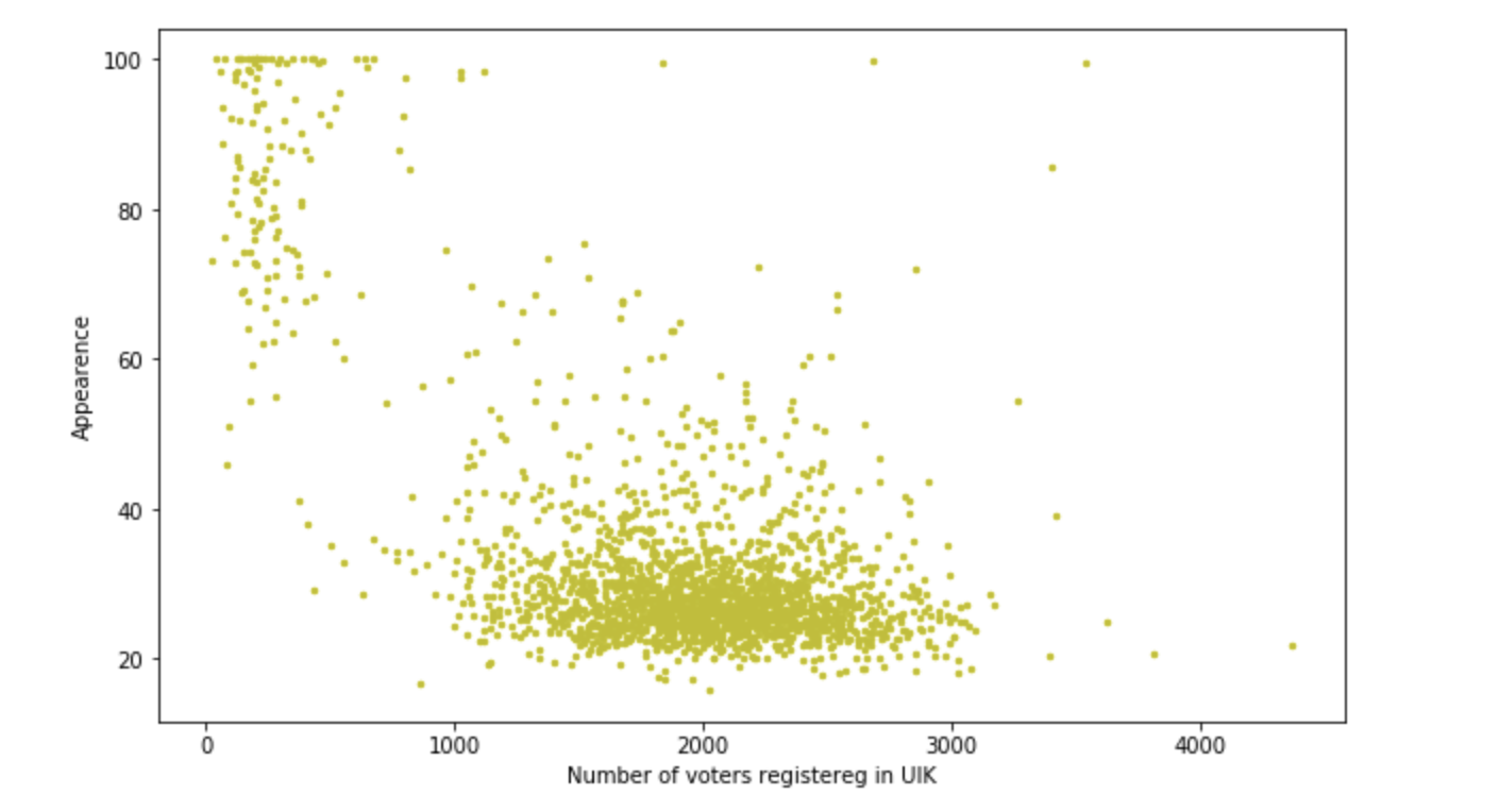
构造是可以忍受的,但是在工作过程中,发现该站点平均有400人,而Beglov的百分比是50到70,但是有两个站点的投票率大于1200,百分比为90 + -0.2。 有趣的是,这发生在这些地区。 有一些出色的搅拌器吗? 还是只开了10人的公共汽车并被迫投票? 我们很高兴地以一种或另一种方式进行了这样的小型调查。 但是我们仍然必须抽牌。 让我们继续。

视觉表示并与Geopandas合作


 ### Extra data for visualization: appearence and number of voters by municipal districts current_UIK = pd.read_html(url, encoding='cp1251', header=0)[7] num_of_voters_dist = [] num_of_voters_voted_dist = [] appearence_dist = [] for j in [num_of_voters_dist, num_of_voters_voted_dist, appearence_dist]: j.extend(0 for i in range (18)) districts = { '0' : [1], # '1' : [2], # '2' : [18], # '3' : [16, 30], # '4' : [10, 14, 22], # '5' : [11, 17], # '6' : [4, 25], # '7' : [5, 24], # '8' : [23, 29], # '9' : [9, 12, 28], # '10' : [13], # '11' : [15], # '12' : [21], # '13' : [20], # '14' : [19, 27], # '15' : [3, 7], # '16' : [6, 26], # '17' : [8] # } for i in districts.keys(): for k in range (1, 31): if k in districts[i]: num_of_voters_dist[int(i)]= num_of_voters_dist[int(i)] + int(current_UIK.iloc[0,k-1]) num_of_voters_voted_dist[int(i)] = num_of_voters_voted_dist[int(i)] + int(current_UIK.iloc[2,k-1]) + int(current_UIK.iloc[3,k-1]) for i in range (18): appearence_dist[i] = round(num_of_voters_voted_dist[i]/num_of_voters_dist[i]*100, 2) 

 ### GeoDataFrame SPb_shapes= gpd.read_file('./shapes/Administrative_Discrits.shp', encoding='cp1251') temp = pd.DataFrame({' ': num_of_voters_dist, '':appearence_dist }) temp[''] = SPb_shapes[['']] temp['geometry'] = SPb_shapes[['geometry']] SPB_elections_visualization = gpd.GeoDataFrame(temp) 

 ### Colored districts SPB_elections_visualization.plot(column = '', linewidth=0, cmap='plasma', legend=True, figsize=[15,15]) 


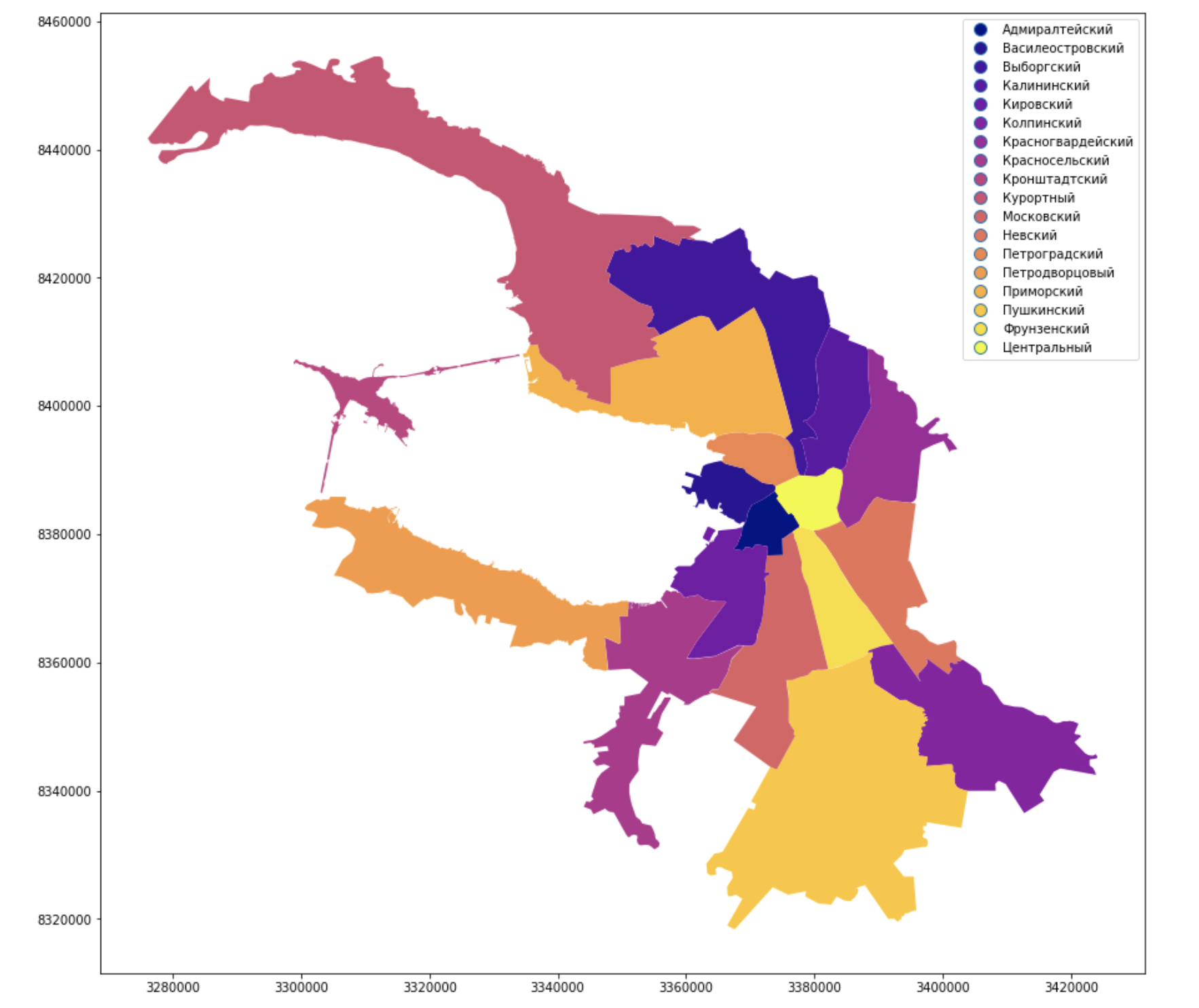
他们给城市的行政区划了油漆并签了字,看起来很熟悉,看起来像彼得,但是涅瓦河还不够。

选民人数

 ### Number of voters gradient SPB_elections_visualization.plot(column = ' ', linewidth=0, cmap='plasma', legend=True, figsize=[15,15]) 


投票率

 ### Appearence gradient SPB_elections_visualization.plot(column = '', linewidth=0, cmap='plasma', legend=True, figsize=[15,15]) 


结论


您可以长时间使用数据,并在不同的领域中使用它,当然,并从中受益,因为它们的存在。 简单而复杂的地理位置可视化工具可以完成很多工作。 在评论中写下您的成功!

Source: https://habr.com/ru/post/zh-CN475258/


All Articles