优化编译器是现代软件的基础:它们允许程序员使用他们理解的语言编写代码,然后将其转换为可由设备有效执行的代码。 优化编译器的任务是了解您编写的输入程序的功能,并创建一个执行相同功能的输出程序,但速度更快。
在本文中,我们将研究优化编译器的一些基本推理技术:如何设计一个程序,使编译器可以轻松工作; 您可以在程序中进行哪些减少以及如何使用它们来减少和加速它。
程序优化器可以在任何地方执行:作为大型编译过程的一个步骤(
Scala Optimizer ); 作为一个单独的程序,在编译器之后和执行之前启动(
Proguard ); 或作为在程序执行期间优化程序的运行时环境的一部分(
JVM JIT编译器 )。 优化器工作的局限性因情况而异,但是它们只有一项任务:采用输入程序并将其转换为输出程序,它执行相同的操作,但是速度更快。
首先,我们将查看程序草案优化的一些示例,以便您了解优化器通常执行的操作以及如何手动执行所有操作。 然后,我们将考虑呈现程序的几种方法,最后,我们将分析可用来分析程序的算法和技术,然后使它们变得更小,更快。
计划草案
所有示例都将用Java给出。 该语言非常普遍,可编译为相对简单的汇编器
-Java Bytecode 。 因此,我们将创建一个良好的基础,借助它,我们可以使用真实的可执行示例探索编译优化技术。 下面介绍的所有技术几乎都可以用于所有其他编程语言。
首先,考虑一个计划草案。 它包含各种逻辑,在过程中注册标准结果并返回计算结果。 该程序本身没有意义,但是将用作说明在保持现有行为的同时可以进行优化的示例:
static int main(int n){ int count = 0, total = 0, multiplied = 0; Logger logger = new PrintLogger(); while(count < n){ count += 1; multiplied *= count; if (multiplied < 100) logger.log(count); total += ackermann(2, 2); total += ackermann(multiplied, n); int d1 = ackermann(n, 1); total += d1 * multiplied; int d2 = ackermann(n, count); if (count % 2 == 0) total += d2; } return total; }
现在,我们假定该程序就是我们所拥有的,代码的其他部分都没有调用它。 它只是将数据输入
main ,执行并返回结果。 现在让我们优化该程序。
优化实例
类型转换和内联
您可能会注意到变量
logger类型不正确:尽管有
Logger标签,但基于代码,我们可以得出结论,这是一个特定的子类
PrintLogger :
- Logger logger = new PrintLogger(); + PrintLogger logger = new PrintLogger();
现在我们知道
logger是
PrintLogger ,并且知道调用
logger.log可以有一个实现。 您可以内联:
- if (multiplied < 100) logger.logcount(); + if (multiplied < 100) System.out.println(count);
这将通过删除不需要的不必要的
ErrLogger类以及删除
public Logger log各种方法来减少程序,因为我们将其内联在调用的单个位置。
凝血常数
在程序执行期间,
count和
total变化,但不
multiplied :它从
0开始,每次都通过
multiplied = multiplied * count ,保持等于
0 。 因此,您可以在整个程序中将其替换为
0 :
static int main(int n){ - int count = 0, total = 0, multiplied = 0; + int count = 0, total = 0; PrintLogger logger = new PrintLogger(); while(count < n){ count += 1; - multiplied *= count; - if (multiplied < 100) System.out.println(count); + if (0 < 100) logger.log(count); total += ackermann(2, 2); - total += ackermann(multiplied, n); + total += ackermann(0, n); int d1 = ackermann(n, 1); - total += d1 * multiplied; int d2 = ackermann(n, count); if (count % 2 == 0) total += d2; } return total; }
结果,我们看到
d1 * multiplied始终为
0 ,这意味着
total += d1 * multiplied不执行任何操作,可以将其删除:
- total += d1 * multiplied
清除死代码
折叠
multiplied并意识到
total += d1 * multiplied无后,您可以删除
int d1的定义:
- int d1 = ackermann(n, 1);
这不再是程序的一部分,并且由于
ackermann是纯函数,因此卸载不会影响程序的结果。
同样,
logger.log联
logger.log ,不再使用
logger本身,可以将其删除:
- PrintLogger logger = new PrintLogger();
移除分支
现在,我们循环中的第一个条件转换取决于
0 < 100 。 由于这始终是正确的,因此您可以简单地删除条件:
- if (0 < 100) System.out.println(count); + System.out.println(count);
任何始终为真的条件转换都可以内联到条件的主体中,对于始终不正确的转换,可以将条件及其主体一起删除。
部分计算
现在,我们分析对
ackermann的三个剩余调用:
total += ackermann(2, 2); total += ackermann(0, n); int d2 = ackermann(n, count);
- 第一个有两个常数。 该函数是纯函数,根据初步计算,
ackermann(2, 2)应该等于7. - 第二个调用具有一个常量参数
0和一个未知n 。 您可以将其传递给ackermann的定义,结果发现,当m为0 ,该函数始终返回n + 1.
- 在第三个调用中,两个参数都是未知的:
n和count 。 让我们暂时保留它们。
鉴于
ackermann的定义如下:
static int ackermann(int m, int n){ if (m == 0) return n + 1; else if (n == 0) return ackermann(m - 1, 1); else return ackermann(m - 1, ackermann(m, n - 1)); }
您可以将其简化为:
- total += ackermann(2, 2); + total += 7 - total += ackermann(0, n); + total += n + 1 int d2 = ackermann(n, count);
延迟排程
d2的定义仅在
if (count % 2 == 0)条件
if (count % 2 == 0) 。 由于
ackermann计算是干净的,因此您可以将此调用转移到条件
ackermann以便在使用之前不对其进行处理:
- int d2 = ackermann(n, count); - if (count % 2 == 0) total += d2; + if (count % 2 == 0) { + int d2 = ackermann(n, count); + total += d2; + }
这将避免对
ackermann(n, count)一半调用,从而加快程序执行速度。
为了进行比较,
System.out.println函数不是干净的,这意味着在不更改程序语义的情况下,无法在条件跳转的内部或外部传递该函数。
优化结果
收集了所有优化之后,我们获得了以下源代码:
static int main(int n){ int count = 0, total = 0; while(count < n){ count += 1; System.out.println(count); total += 7; total += n + 1; if (count % 2 == 0) { total += d2; int d2 = ackermann(n, count); } } return total; } static int ackermann(int m, int n){ if (m == 0) return n + 1; else if (n == 0) return ackermann(m - 1, 1); else return ackermann(m - 1, ackermann(m, n - 1)); }
尽管我们已经手动进行了优化,但是所有这些都可以自动完成。 以下是我为JVM程序编写的原型优化器的反编译结果:
static int main(int var0) { new Demo.PrintLogger(); int var1 = 0; int var3; for(int var2 = 0; var2 < var0; var2 = var3) { System.out.println(var3 = 1 + var2); int var10000 = var3 % 2; int var7 = var1 + 7 + var0 + 1; var1 = var10000 == 0 ? var7 + ackermann(var0, var3) : var7; } return var1; } static int ackermann__I__TI1__I(int var0) { if (var0 == 0) return 2; else return ackermann(var0 - 1, var0 == 0 ? 1 : ackermann__I__TI1__I(var0 - 1);); } static int ackermann(int var0, int var1) { if (var0 == 0) return var1 + 1; else return var1 == 0 ? ackermann__I__TI1__I(var0 - 1) : ackermann(var0 - 1, ackermann(var0, var1 - 1)); } static class PrintLogger implements Demo.Logger {} interface Logger {}
反编译的代码与手动优化的版本略有不同。 编译器无法优化的某些内容(例如,未使用的对
new PrintLogger调用),但是做了一些不同的事情(例如,
ackermann和
ackermann__I__TI1__I )。 但是对于其余部分,自动优化器使用嵌入在其中的逻辑与我做相同的事情。
问题出现了:如何?
中级意见
如果您尝试创建自己的优化器,那么出现的第一个问题也许是最重要的:什么是“程序”?
毫无疑问,您习惯于以源代码的形式编写和更改程序。 您肯定以编译二进制文件的形式执行了它们,甚至调试了二进制文件。 您可能会以
语法树 ,
三地址代码 ,
A-Normal ,
Continuation Passing Style或
Single Static Assignment的形式遇到程序。
有一个由不同程序表示的整个动物园。 在这里,我们将讨论在优化器中表示“程序”的最重要方法。
源代码
static int ackermann(int m, int n){ if (m == 0) return n + 1; else if (n == 0) return ackermann(m - 1, 1); else return ackermann(m - 1, ackermann(m, n - 1)); }
未编译的源代码也表示您的程序。 它相对紧凑,易于阅读,但是有两个缺点:
- 源代码包含名称和格式的所有详细信息,这对程序员很重要,但对计算机却没有用。
- 源代码形式的错误程序要比正确的程序多得多,并且在优化过程中,您需要确保将程序从正确的输入源代码转换为正确的输出源代码。
这些因素使优化器难以以源代码的形式使用程序。 是的,您
可以转换这样的程序,例如,使用
正则表达式来识别和替换模式。 但是,两个因素中的第一个因素使得难以可靠地识别带有大量无关细节的模式。 第二个因素极大地增加了混淆和获取错误程序的可能性。
这些限制对于在人工监督下执行的程序转换器是可以接受的,例如,当您可以使用
Codemod重构和转换代码库时。 但是,您不能将源代码用作自动化优化器的主要模型。
抽象语法树
static int ackermann(int m, int n){ if (m == 0) return n + 1; else if (n == 0) return ackermann(m - 1, 1); else return ackermann(m - 1, ackermann(m, n - 1)); } IfElse( cond = BinOp(Ident("m"), "=", Literal(0)), then = Return(BinOp(Ident("n"), "+", Literal(1)), else = IfElse( cond = BinOp(Ident("n"), "=", Literal(0)), then = Return(Call("ackermann", BinOp(Ident("m"), "-", Literal(1)), Literal(1)), else = Return( Call( "ackermann", BinOp(Ident("m"), "-", Literal(1)), Call("ackermann", Ident("m"), BinOp(Ident("n"), "-", Literal(1))) ) ) ) )

抽象语法树(AST)是另一种常见的中间格式。 与源代码相比,它们位于抽象阶梯的下一步。 通常,AST丢弃所有源代码格式,缩进和注释,但保留以更抽象的表示形式丢弃的局部变量的名称。
像源代码一样,AST也可能会编码不影响程序实际语义的不必要信息。 例如,以下两个代码片段在语义上是相同的; 它们仅在局部变量的名称上有所不同,但仍具有不同的AST:
static int ackermannA(int m, int n){ int p = n; int q = m; if (q == 0) return p + 1; else if (p == 0) return ackermannA(q - 1, 1); else return ackermannA(q - 1, ackermannA(q, p - 1)); } Block( Assign("p", Ident("n")), Assign("q", Ident("m")), IfElse( cond = BinOp(Ident("q"), "==", Literal(0)), then = Return(BinOp(Ident("p"), "+", Literal(1)), else = IfElse( cond = BinOp(Ident("p"), "==", Literal(0)), then = Return(Call("ackermann", BinOp(Ident("q"), "-", Literal(1)), Literal(1)), else = Return( Call( "ackermann", BinOp(Ident("q"), "-", Literal(1)), Call("ackermann", Ident("q"), BinOp(Ident("p"), "-", Literal(1))) ) ) ) ) ) static int ackermannB(int m, int n){ int r = n; int s = m; if (s == 0) return r + 1; else if (r == 0) return ackermannB(s - 1, 1); else return ackermannB(s - 1, ackermannB(s, r - 1)); } Block( Assign("r", Ident("n")), Assign("s", Ident("m")), IfElse( cond = BinOp(Ident("s"), "==", Literal(0)), then = Return(BinOp(Ident("r"), "+", Literal(1)), else = IfElse( cond = BinOp(Ident("r"), "==", Literal(0)), then = Return(Call("ackermann", BinOp(Ident("s"), "-", Literal(1)), Literal(1)), else = Return( Call( "ackermann", BinOp(Ident("s"), "-", Literal(1)), Call("ackermann", Ident("s"), BinOp(Ident("r"), "-", Literal(1))) ) ) ) ) )
关键在于,尽管AST具有树结构,但它们包含在语义上不像树的节点:
Ident("r")和
Ident("s")值不是由其子树的内容确定的,而是由上游的
Assign("r", ...)节点)确定的
Assign("r", ...)和
Assign("s", ...) 。 实际上,
Ident和
Assign之间还有其他语义关系,与AST树结构中的边同样重要:

这些连接形成通用的图结构,包括函数递归定义存在时的循环。
字节码
由于我们选择Java作为主要语言,因此编译后的程序将作为Java字节码保存在.class文件中。
回想一下我们的
ackermann函数:
static int ackermann(int m, int n){ if (m == 0) return n + 1; else if (n == 0) return ackermann(m - 1, 1); else return ackermann(m - 1, ackermann(m, n - 1)); }
它编译为以下字节码:
0: iload_0 1: ifne 8 4: iload_1 5: iconst_1 6: iadd 7: ireturn 8: iload_1 9: ifne 20 12: iload_0 13: iconst_1 14: isub 15: iconst_1 16: invokestatic ackermann:(II)I 19: ireturn 20: iload_0 21: iconst_1 22: isub 23: iload_0 24: iload_1 25: iconst_1 26: isub 27: invokestatic ackermann:(II)I 30: invokestatic ackermann:(II)I 33: ireturn
运行Java字节码的Java虚拟机(JVM)是一台具有堆栈和寄存器的组合的计算机:有一个操作数堆栈(STACK),在其中操作值,还有一个局部变量(LOCALS),可以在其中存储这些值。 该函数以局部变量的前N个插槽中的N个参数开头。 在执行时,函数将数据移到堆栈上,对其进行操作,然后将其放回变量中,然后调用return将值从操作数堆栈返回给调用方。
如果注释上面的字节码以表示在堆栈和局部变量表之间移动的值,则它将看起来像这样:
BYTECODE LOCALS STACK |a0|a1| | 0: iload_0 |a0|a1| |a0| 1: ifne 8 |a0|a1| | 4: iload_1 |a0|a1| |a1| 5: iconst_1 |a0|a1| |a1| 1| 6: iadd |a0|a1| |v1| 7: ireturn |a0|a1| | 8: iload_1 |a0|a1| |a1| 9: ifne 20 |a0|a1| | 12: iload_0 |a0|a1| |a0| 13: iconst_1 |a0|a1| |a0| 1| 14: isub |a0|a1| |v2| 15: iconst_1 |a0|a1| |v2| 1| 16: invokestatic ackermann:(II)I |a0|a1| |v3| 19: ireturn |a0|a1| | 20: iload_0 |a0|a1| |a0| 21: iconst_1 |a0|a1| |a0| 1| 22: isub |a0|a1| |v4| 23: iload_0 |a0|a1| |v4|a0| 24: iload_1 |a0|a1| |v4|a0|a1| 25: iconst_1 |a0|a1| |v4|a0|a1| 1| 26: isub |a0|a1| |v4|a0|v5| 27: invokestatic ackermann:(II)I |a0|a1| |v4|v6| 30: invokestatic ackermann:(II)I |a0|a1| |v7| 33: ireturn |a0|a1| |
在这里,
a1使用
a0和
a1向函数提供了参数,这些参数存储在函数的最开始的LOCALS表中。
1表示通过
iconst_1加载的
iconst_1 ,以及从
v1到
v7计算中间值。 有三个
ireturn指令返回
v1 ,
v3和
v7 。 此函数未定义其他局部变量,因此LOCALS数组仅存储输入参数。
上面,我们看到了函数的两个变体
ackermannA和
ackermannB 。 所以他们看字节码:
BYTECODE LOCALS STACK |a0|a1| | 0: iload_1 |a0|a1| |a1| 1: istore_2 |a0|a1|a1| | 2: iload_0 |a0|a1|a1| |a0| 3: istore_3 |a0|a1|a1|a0| | 4: iload_3 |a0|a1|a1|a0| |a0| 5: ifne 12 |a0|a1|a1|a0| | 8: iload_2 |a0|a1|a1|a0| |a1| 9: iconst_1 |a0|a1|a1|a0| |a1| 1| 10: iadd |a0|a1|a1|a0| |v1| 11: ireturn |a0|a1|a1|a0| | 12: iload_2 |a0|a1|a1|a0| |a1| 13: ifne 24 |a0|a1|a1|a0| | 16: iload_3 |a0|a1|a1|a0| |a0| 17: iconst_1 |a0|a1|a1|a0| |a0| 1| 18: isub |a0|a1|a1|a0| |v2| 19: iconst_1 |a0|a1|a1|a0| |v2| 1| 20: invokestatic ackermannA:(II)I |a0|a1|a1|a0| |v3| 23: ireturn |a0|a1|a1|a0| | 24: iload_3 |a0|a1|a1|a0| |a0| 25: iconst_1 |a0|a1|a1|a0| |a0| 1| 26: isub |a0|a1|a1|a0| |v4| 27: iload_3 |a0|a1|a1|a0| |v4|a0| 28: iload_2 |a0|a1|a1|a0| |v4|a0|a1| 29: iconst_1 |a0|a1|a1|a0| |v4|a0|a1| 1| 30: isub |a0|a1|a1|a0| |v4|a0|v5| 31: invokestatic ackermannA:(II)I |a0|a1|a1|a0| |v4|v6| 34: invokestatic ackermannA:(II)I |a0|a1|a1|a0| |v7| 37: ireturn |a0|a1|a1|a0| |
由于源代码接受两个参数并将它们放在局部变量中,因此字节码具有相应的指令,可从本地索引0和1加载参数值并将其保存在索引2和3下。但是,字节码对局部变量的名称不感兴趣:它可与与LOCALS数组中的索引完全相同。 因此,
ackermannA和
ackermannB将具有相同的字节码。 这是合乎逻辑的,因为它们在语义上是等效的!
但是,
ackermannA和
ackermannB不能与原始
ackermann编译到相同的字节码中:尽管字节码是从局部变量的名称中抽象出来的,但是从加载和保存到这些变量或从这些变量中保存后,它仍然没有完全抽象出来。 尽管这些值不会影响程序的实际行为,但对我们来说仍然很重要。
除了缺乏从加载/保存中抽象的概念外,字节码还有另一个缺点:像大多数线性汇编程序一样,它在紧凑性方面进行了非常优化,在进行优化时很难修改它。
为了更清楚,让我们看一下原始
ackermann函数的字节码:
BYTECODE LOCALS STACK |a0|a1| | 0: iload_0 |a0|a1| |a0| 1: ifne 8 |a0|a1| | 4: iload_1 |a0|a1| |a1| 5: iconst_1 |a0|a1| |a1| 1| 6: iadd |a0|a1| |v1| 7: ireturn |a0|a1| | 8: iload_1 |a0|a1| |a1| 9: ifne 20 |a0|a1| | 12: iload_0 |a0|a1| |a0| 13: iconst_1 |a0|a1| |a0| 1| 14: isub |a0|a1| |v2| 15: iconst_1 |a0|a1| |v2| 1| 16: invokestatic ackermann:(II)I |a0|a1| |v3| 19: ireturn |a0|a1| | 20: iload_0 |a0|a1| |a0| 21: iconst_1 |a0|a1| |a0| 1| 22: isub |a0|a1| |v4| 23: iload_0 |a0|a1| |v4|a0| 24: iload_1 |a0|a1| |v4|a0|a1| 25: iconst_1 |a0|a1| |v4|a0|a1| 1| 26: isub |a0|a1| |v4|a0|v5| 27: invokestatic ackermann:(II)I |a0|a1| |v4|v6| 30: invokestatic ackermann:(II)I |a0|a1| |v7| 33: ireturn |a0|a1| |
让我们进行一个粗略的更改:让函数调用
30: invokestatic ackermann:(II)I不使用它的第一个参数。 然后可以用等效的调用
30: invokestatic ackermann2:(I)I代替此调用
30: invokestatic ackermann2:(I)I ,它仅接受一个参数。 这是一个常见的优化,它允许使用“死代码删除”来抛出用于计算第一个参数的任何代码
30: invokestatic ackermann:(II)I为此,我们不仅需要替换指令
30 ,还需要查看指令列表,了解第一个参数的计算位置(
STACK v4 ),并将其删除。 我们从指令
30返回到
22 ,从指令
22返回到
21和
20 。 最终版本:
BYTECODE LOCALS STACK |a0|a1| | 0: iload_0 |a0|a1| |a0| 1: ifne 8 |a0|a1| | 4: iload_1 |a0|a1| |a1| 5: iconst_1 |a0|a1| |a1| 1| 6: iadd |a0|a1| |v1| 7: ireturn |a0|a1| | 8: iload_1 |a0|a1| |a1| 9: ifne 20 |a0|a1| | 12: iload_0 |a0|a1| |a0| 13: iconst_1 |a0|a1| |a0| 1| 14: isub |a0|a1| |v2| 15: iconst_1 |a0|a1| |v2| 1| 16: invokestatic ackermann:(II)I |a0|a1| |v3| 19: ireturn |a0|a1| | - 20: iload_0 |a0|a1| | - 21: iconst_1 |a0|a1| | - 22: isub |a0|a1| | 23: iload_0 |a0|a1| |a0| 24: iload_1 |a0|a1| |a0|a1| 25: iconst_1 |a0|a1| |a0|a1| 1| 26: isub |a0|a1| |a0|v5| 27: invokestatic ackermann:(II)I |a0|a1| |v6| - 30: invokestatic ackermann:(II)I |a0|a1| |v7| + 30: invokestatic ackermann2:(I)I |a0|a1| |v7| 33: ireturn |a0|a1| |
我们仍然可以对简单的
ackermann函数进行如此简单的更改。 但是,在实际项目中使用的大型功能中,进行大量相互关联的更改将变得更加困难。 通常,对程序进行的任何小的语义更改都可能需要在整个字节码中进行大量更改。
您可能会注意到,我们通过分析LOCALS和STACK中的值进行了上述更改:我们观察了如何将
v4从指令
22传递给指令
30 ,以及
22将数据从
a0指令
21和
20传递给
a0和
1 。 这些值根据图形原理在LOCALS和STACK之间传输:从计算该值的指令到其进一步使用的地方。
像我们的AST中的“
Ident /
Assign对一样,在LOCALS和STACK之间传递的值在值的计算点与使用点之间形成了一个图形。 那么,为什么不开始直接使用图形呢?
数据流图
数据流图是继字节码之后的下一个抽象级别。 如果使用
Ident /
Assign关系扩展语法树,或者跟踪字节码如何在LOCALS和STACK之间移动值,则可以构建图形。 对于
ackermann函数
ackermann它看起来像这样:

与AST或Java堆栈字节码字节码不同,数据流图不使用“局部变量”的概念:相反,该图包含每个值与其使用位置之间的直接连接。 分析字节码时,通常需要抽象解释LOCALS和STACK以便了解值的移动方式。 AST分析包括跟踪树并使用包含
Assign /
Ident关联的符号表; 分析数据流图通常是对转换的直接跟踪-“移动值”的纯净想法,而无需提供程序的外壳。
ackermann也比线性字节码更易于操作:用
ackermann调用替换为
ackermann调用的节点并
ackermann2其中一个参数只是更改图节点(标记为绿色)并删除输入链接之一和传递节点(标记为红色):

如您所见,程序中的微小变化(用
ackermann(int n, int m)替换
ackermann(int n, int m) ackermann2(int m) )变成了数据流图中相对本地化的变化。
通常,使用图形比使用线性字节码或AST要容易得多:它们易于分析和更改。
图的描述中没有太多细节:除了图的实际物理表示之外,还有许多其他的状态和流控制建模方法,这些方法在本文的范围之内甚至更困难。 我还省略了许多有关转换图形的细节,例如,添加和删除链接,正向和反向过渡,水平和垂直过渡(在宽度和深度上)等。如果您研究了算法,那么您应该对所有这些都熟悉。
最后,我们省略了从线性字节码到图形,然后从图形回到字节码的转换算法。 这本身是一项有趣的任务,但我们将其留给您进行独立研究。
分析方法
在了解了程序的思想之后,我们需要对其进行分析:找出一些事实,这些事实将使您能够在不更改程序行为的情况下对其进行转换。 上面讨论的许多优化都是基于对该程序的分析:
- 常量折叠:表达式的结果是否为已知的常量值? 表达式计算是否纯净?
- 类型转换和内联:方法调用类型是否是具有被调用方法的单个实现的类型?
- : ?
- : «»? - ? ?
- : , ?
, , , . , , , .
, , , — , . .
(Inference Lattice)
, . , «» - :
Integer ? String ? Array[Float] ? PrintLogger ?
CharSequence ? String , - StringBuilder ?
Any , , ?
:

: ,
"hello" String ,
String CharSequence .
"hello" , (Singleton Type) — . :

, , . , . , , ,
String StringBuilder , , :
CharSequence . ,
0 ,
1 ,
2 , ,
Integer .

, , :

, , . , .
count
main :
static int main(int n){ int count = 0, multiplied = 0; while(count < n){ if (multiplied < 100) logger.log(count); count += 1; multiplied *= count; } return ...; }
ackermann ,
count ,
multiplied logger . :

,
count 0 block0 .
block1 , ,
count < n : ,
block3 return ,
block2 ,
count 1 count ,
block1 . ,
< false ,
block3 .
?
block0 . , count = 0.
block1 , , n ( , Integer ), , if . block2 block3.block3 , , block1b , block2 , , block1c . , block2 count , 1 count.- ,
count 0 1 : count Integer. - :
block1 n count Integer .
block2 , count Integer + 1 -> Integer . , count Integer , .
multiplied
,
multiplied :
block0 . , multiplied 0.
block1 , , . block2 block3 ( ).
block2 , block2 ( 0 ) count ( Integer ). 0 * Integer -> 0 , multiplied 0.
block1 block2 . multiplied 0 , .
multiplied 0 , , :
multiplied < 100 true.
if (multiplied < 100) logger.log(count); logger.log(count) .
- ,
multiplied , , 0 .
:

:

:
static int main(int n){ int count = 0; while(count < n){ logger.log(count); count += 1; } return ...; }
, , , , .
multiplied -> 0 , , . , , . , .
, . :
count ,
multiplied . ,
multiplied count ,
count multiplied . , .
, — : , . , ( ) . .
while , ,
O( ) . (, ) , , .
, .
, . , , , , .
. :
static int main(int n){ return called(n, 0); } static int called(int x, int y){ return x * y; }
:

main :
main(n)
called(n, 0)
called(n, 0) 0
main(n) 0
, , . .
,
called(n, 0) 0 , :

:
static int main(int n){ return 0; }
: A B, C, D, D C, B, D A. A B B A, A A, , !
, Java:
public static Any factorial(int n) { if (n == 1) { return 1; } else { return n * factorial(n - 1); } }
n int ,
Any : . ,
factorial int (
Integer ).
factorial ,
factorial factorial , ! ?
Bottom
Bottom :

« , , ».
Bottom factorial :

block0 . n Integer , 1 1 , n == 1 , true false .
true : return 1 .
false n - 1 n Integer .
factorial — , Bottom .
* n: Integer factorial : Bottom Bottom .
return Bottom .factorial 1 Bottom , 1 .
1 factorial , Bottom .
Integer * 1 Integer .
return Integer .factorial Integer 1 , Integer .
factorial , Integer . * n: Integer factorial: Integer , Integer , .
factorial Integer , , .
, .
Bottom , , .
* :
(n: Integer) * (factorial: Bottom)
(n: Integer) * (factorial: 1)
(n: Integer) * (factorial: Integer)
multiplied ,
O( ) . , , .
— , « ». , (« »), , (« »). .
main :
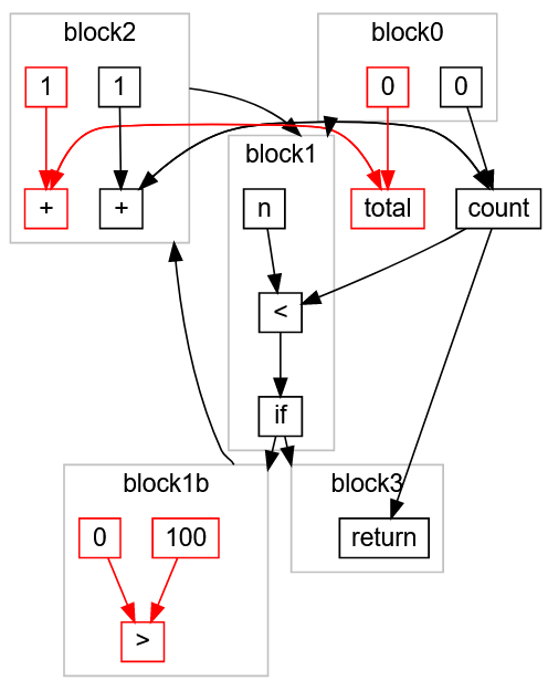
static int main(int n){ int count = 0, total = 0, multiplied = 0; while(count < n){ if (multiplied > 100) count += 1; count += 1; multiplied *= 2; total += 1; } return count; }
,
if (multiplied > 100) multiplied *= count multiplied *= 2 . .
, :
multiplied > 100 true , count += 1 («»).
total , («»).
, :
static int main(int n){ int count = 0; while(count < n){ count += 1; } return count; }
, .
:

, , :
block0 ,
block1 , ,
block1b , ,
block1c , ,
return block3 .
,
multiplied -> 0 , :

:

,
block1b (
0 > 100 )
true .
false block1c (
if ):
, « »
total > , - , , . ,
return ,
:
> ,
100 ,
0 block1b ,
total ,
0 ,
+ 1 ,
total block0 block2 . :

«» :
static int main(int n){ int count = 0; while(count < n){ count += 1; } return count; }
结论
:
- -.
- , .
- , . .
- : «» «» , , .
- : , .
- , .
, , .
, . . , :