本文的目的是教导神经网络玩“人生”游戏而不讲授游戏规则。
哈Ha! 我向您介绍了kylewbanks的文章“使用卷积神经网络与 Keras 玩Conway的生活游戏”的翻译。
如果您不熟悉名为Life的游戏( 这是英国数学家John Conway在1970年发明的细胞自动机 ),则规则如下。
游戏世界是一个无限的二维正方形网格,每个正方形网格处于两种可能的状态之一:活着或死了(分别是有人居住和无人居住)。 每个像元与其水平,垂直或对角线的八个邻居互动。 在每个时间步上,都会发生以下转换:
- 少于两个活体邻居的任何活细胞都会死亡。
- 任何有两个或三个活着邻居的活细胞都可以存活到下一代。
- 任何具有三个以上活着邻居的活细胞都会死亡。
- 任何具有三个活着邻居的死细胞都将成为一个活细胞。
第一代是通过将上述规则同时应用于初始状态的每个单元格来创建的,出生和死亡同时发生在离散的时间点。 每一代都是上一代的纯粹功能。 该规则继续适用于新一代,以创建下一代。
有关详细信息,请参见Wikipedia 。
为什么这样 主要用于娱乐,并了解一些关于卷积神经网络的知识。
所以...
游戏逻辑
首先要做的是定义一个函数,该函数将比赛场地作为输入并返回下一个状态。
幸运的是,Internet上有许多实现,例如: https : //jakevdp.imtqy.com/blog/2013/08/07/conways-game-of-life/ 。
实际上,它以比赛场的矩阵作为输入,其中0表示死单元,而1表示活单元,并返回相同大小的矩阵,但包含游戏的下一次迭代中每个单元的状态。
import numpy as np def life_step(X): live_neighbors = sum(np.roll(np.roll(X, i, 0), j, 1) for i in (-1, 0, 1) for j in (-1, 0, 1) if (i != 0 or j != 0)) return (live_neighbors == 3) | (X & (live_neighbors == 2)).astype(int)
运动场的产生
按照游戏逻辑,我们需要一种随机生成游戏场的方法以及一种可视化它们的方法。
generate_frames函数创建具有一定形状和每个单元格将处于“活动”状态的预定概率num_frames随机游戏场的num_frames , render_frames绘制两个游戏场的图像表示以进行比较(活动单元格为白色,死单元格为黑色):
import matplotlib.pyplot as plt def generate_frames(num_frames, board_shape=(100,100), prob_alive=0.15): return np.array([ np.random.choice([False, True], size=board_shape, p=[1-prob_alive, prob_alive]) for _ in range(num_frames) ]).astype(int) def render_frames(frame1, frame2): plt.subplot(1, 2, 1) plt.imshow(frame1.flatten().reshape(board_shape), cmap='gray') plt.subplot(1, 2, 2) plt.imshow(frame2.flatten().reshape(board_shape), cmap='gray')
让我们看看这些字段是什么样的:
board_shape = (20, 20) board_size = board_shape[0] * board_shape[1] probability_alive = 0.15 frames = generate_frames(10, board_shape=board_shape, prob_alive=probability_alive) print(frames.shape)
(10, 20, 20)
print(frames[0])
[[0, 0, 0, 1, 0, 0, 1, 1, 0, 0, 1, 0, 0, 0, 1, 0, 0, 0, 1, 0], [0, 0, 0, 0, 1, 0, 0, 0, 0, 0, 0, 1, 0, 0, 0, 0, 0, 0, 1, 1], [0, 0, 0, 0, 0, 0, 0, 0, 0, 0, 0, 0, 1, 0, 1, 0, 1, 0, 0, 0], [0, 0, 0, 0, 0, 0, 0, 0, 0, 0, 0, 0, 0, 0, 1, 0, 1, 0, 0, 0], [0, 0, 0, 0, 0, 0, 0, 0, 0, 0, 0, 0, 0, 0, 1, 0, 0, 0, 0, 0], [0, 1, 0, 0, 0, 0, 0, 1, 0, 1, 0, 0, 0, 0, 0, 0, 0, 0, 0, 0], [0, 0, 0, 0, 0, 0, 0, 0, 0, 0, 0, 0, 0, 0, 0, 0, 0, 0, 0, 0], [0, 0, 0, 0, 0, 0, 0, 0, 0, 0, 0, 0, 0, 0, 0, 0, 0, 0, 0, 0], [0, 0, 0, 0, 0, 0, 0, 0, 0, 0, 1, 0, 0, 0, 1, 0, 0, 0, 0, 1], [0, 0, 0, 0, 0, 0, 0, 0, 0, 0, 1, 0, 0, 0, 0, 0, 1, 0, 1, 1], [1, 0, 0, 0, 1, 0, 1, 0, 0, 0, 1, 0, 0, 0, 0, 0, 0, 0, 0, 0], [0, 0, 0, 0, 0, 1, 0, 0, 1, 1, 0, 0, 0, 0, 0, 0, 1, 0, 0, 0], [1, 0, 0, 0, 0, 1, 1, 0, 0, 0, 0, 0, 0, 0, 1, 0, 0, 0, 0, 0], [0, 0, 0, 0, 0, 0, 0, 1, 0, 0, 1, 0, 0, 0, 0, 1, 1, 0, 0, 0], [0, 0, 1, 0, 0, 1, 0, 0, 0, 0, 0, 0, 0, 0, 0, 0, 0, 0, 0, 0], [0, 0, 0, 0, 0, 0, 1, 0, 0, 0, 0, 0, 0, 0, 1, 0, 0, 0, 0, 0], [0, 0, 0, 0, 0, 0, 1, 0, 0, 0, 0, 1, 1, 1, 1, 0, 0, 0, 0, 0], [0, 0, 1, 0, 0, 0, 0, 0, 0, 0, 0, 0, 1, 0, 0, 0, 0, 0, 0, 0], [0, 0, 0, 1, 0, 0, 0, 1, 1, 0, 0, 0, 0, 0, 1, 0, 0, 0, 0, 0], [0, 0, 1, 0, 0, 0, 0, 0, 0, 0, 0, 0, 0, 0, 1, 0, 1, 0, 1, 0]])
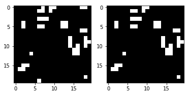
接下来,获取比赛场地的整数表示并将其显示为图像。
使用life_step函数还在右侧显示了运动场的以下状态:
ender_frames(frames[1], life_step(frames[1]))

建立培训和测试集
现在,我们可以生成用于培训,验证和测试的数据。
y_train / y_val / y_test中的每个元素将代表y_train / y_val / y_test该字段每一帧的下一个游戏字段。
def reshape_input(X): return X.reshape(X.shape[0], X.shape[1], X.shape[2], 1) def generate_dataset(num_frames, board_shape, prob_alive): X = generate_frames(num_frames, board_shape=board_shape, prob_alive=prob_alive) X = reshape_input(X) y = np.array([ life_step(frame) for frame in X ]) return X, y train_size = 70000 val_size = 10000 test_size = 20000
print("Training Set:") X_train, y_train = generate_dataset(train_size, board_shape, probability_alive) print(X_train.shape) print(y_train.shape)
Training Set: (70000, 20, 20, 1) (70000, 20, 20, 1)
print("Validation Set:") X_val, y_val = generate_dataset(val_size, board_shape, probability_alive) print(X_val.shape) print(y_val.shape)
Validation Set: (10000, 20, 20, 1) (10000, 20, 20, 1)
print("Test Set:") X_test, y_test = generate_dataset(test_size, board_shape, probability_alive) print(X_test.shape) print(y_test.shape)
Test Set: (20000, 20, 20, 1) (20000, 20, 20, 1)
卷积神经网络构造
现在,我们可以迈出使用Keras构建卷积神经网络的第一步。 这里的关键是内核大小(3、3)和第1步。它们告诉CNN为它要查看的字段中的每个单元(包括当前单元)使用周围单元的3x3矩阵。
例如,如果下面是游戏场,并且我们在x的中间单元格中,她将查看所有标有感叹号的单元格! 和单元格
0 0 0 0 0 0! ! ! 0 0! x ! 0 0! ! ! 0 0 0 0 0 0
网络的其余部分非常简单,因此我不再赘述。 如果您对任何内容都感兴趣,建议阅读文档。
from keras.models import Sequential from keras.layers import Dense, Dropout, Activation, Conv2D, MaxPool2D
看一下summary函数的输出:
model.summary()
_________________________________________________________________ Layer (type) Output Shape Param # ================================================================= conv2d_9 (Conv2D) (None, 20, 20, 50) 500 _________________________________________________________________ dense_17 (Dense) (None, 20, 20, 100) 5100 _________________________________________________________________ dense_18 (Dense) (None, 20, 20, 1) 101 _________________________________________________________________ activation_9 (Activation) (None, 20, 20, 1) 0 ================================================================= Total params: 5,701 Trainable params: 5,701 Non-trainable params: 0 _________________________________________________________________
训练并保存模型
构建了CNN之后,让我们训练模型并将其保存到磁盘:
def train(model, X_train, y_train, X_val, y_val, batch_size=50, epochs=2, filename_suffix=''): model.fit( X_train, y_train, batch_size=batch_size, epochs=epochs, validation_data=(X_val, y_val) ) with open('cgol_cnn{}.json'.format(filename_suffix), 'w') as file: file.write(model.to_json()) model.save_weights('cgol_cnn{}.h5'.format(filename_suffix)) train(model, X_train, y_train, X_val, y_val, filename_suffix='_basic')
Train on 70000 samples, validate on 10000 samples Epoch 1/2 70000/70000 [==============================] - 27s 388us/step - loss: 0.1324 - acc: 0.9651 - val_loss: 0.0833 - val_acc: 0.9815 Epoch 2/2 70000/70000 [==============================] - 27s 383us/step - loss: 0.0819 - acc: 0.9817 - val_loss: 0.0823 - val_acc: 0.9816
该模型为训练集和测试集提供了超过98%的准确性,这对于首次通过非常好。 让我们尝试找出我们犯错的地方。
试一下
让我们看一下随机竞争环境的预测及其工作原理。 首先,创建一个运动场并查看正确的下一帧:
X, y = generate_dataset(1, board_shape=board_shape, prob_alive=probability_alive) render_frames(X[0].flatten().reshape(board_shape), y)

接下来,让我们进行预测,看看有多少个单元格被错误地预测:
pred = model.predict_classes(X) print(np.count_nonzero(pred.flatten() - y.flatten()), "incorrect cells.")
4 incorrect cells.
接下来,让我们将正确的下一步与预测的步骤进行比较:
render_frames(y, pred.flatten().reshape(board_shape))
这并不可怕,但是您看到预测失败的地方了吗? 网络似乎无法预测运动场边缘的单元。 让我们看看非零值表示不正确的预测的地方:
print(pred.flatten().reshape(board_shape) - y.flatten().reshape(board_shape))
[[ 0 0 0 0 0 0 0 -1 0 0 0 0 0 0 0 0 0 -1 -1 0] [ 0 0 0 0 0 0 0 0 0 0 0 0 0 0 0 0 0 0 0 0] [ 0 0 0 0 0 0 0 0 0 0 0 0 0 0 0 0 0 0 0 0] [ 0 0 0 0 0 0 0 0 0 0 0 0 0 0 0 0 0 0 0 0] [ 0 0 0 0 0 0 0 0 0 0 0 0 0 0 0 0 0 0 0 0] [ 0 0 0 0 0 0 0 0 0 0 0 0 0 0 0 0 0 0 0 0] [ 0 0 0 0 0 0 0 0 0 0 0 0 0 0 0 0 0 0 0 0] [ 0 0 0 0 0 0 0 0 0 0 0 0 0 0 0 0 0 0 0 0] [ 0 0 0 0 0 0 0 0 0 0 0 0 0 0 0 0 0 0 0 0] [ 0 0 0 0 0 0 0 0 0 0 0 0 0 0 0 0 0 0 0 0] [ 0 0 0 0 0 0 0 0 0 0 0 0 0 0 0 0 0 0 0 0] [ 0 0 0 0 0 0 0 0 0 0 0 0 0 0 0 0 0 0 0 0] [ 0 0 0 0 0 0 0 0 0 0 0 0 0 0 0 0 0 0 0 0] [ 0 0 0 0 0 0 0 0 0 0 0 0 0 0 0 0 0 0 0 0] [ 0 0 0 0 0 0 0 0 0 0 0 0 0 0 0 0 0 0 0 0] [ 0 0 0 0 0 0 0 0 0 0 0 0 0 0 0 0 0 0 0 0] [ 0 0 0 0 0 0 0 0 0 0 0 0 0 0 0 0 0 0 0 0] [ 0 0 0 0 0 0 0 0 0 0 0 0 0 0 0 0 0 0 0 0] [ 0 0 0 0 0 0 0 0 0 0 0 0 0 0 0 0 0 0 0 0] [ 0 0 0 0 0 0 -1 0 0 0 0 0 0 0 0 0 0 0 0 0]]
如您所见,所有非零值都位于运动场的边缘。 让我们看一下完整的测试套件,并确认此观察是正确的。
使用测试套件查看错误
我们将编写一个显示热图的函数,以显示模型在哪里出错,并使用整个测试套件进行调用:
def view_prediction_errors(model, X, y): y_pred = model.predict_classes(X) sum_y_pred = np.sum(y_pred, axis=0).flatten().reshape(board_shape) sum_y = np.sum(y, axis=0).flatten().reshape(board_shape) plt.imshow(sum_y_pred - sum_y, cmap='hot', interpolation='nearest') plt.show() view_prediction_errors(model, X_test, y_test)

在边缘和角落的所有错误。 这是合乎逻辑的,因为CNN不能环顾四周,但是life_step中游戏的逻辑life_step做到这一点。 例如,请考虑以下内容。 查看下方的边缘单元x ,CNN仅看到x和! 单元格:
0 0 0 0 0 ! ! 0 0 0 x ! 0 0 0 ! ! 0 0 0 0 0 0 0 0
但是我们真正想要的和life_step所做的是life_step看单元格:
0 0 0 0 0 ! ! 0 0 ! x ! 0 0 ! ! ! 0 0 ! 0 0 0 0 0
拐角处的情况类似:
x ! 0 0 ! ! ! 0 0 ! 0 0 0 0 0 0 0 0 0 0 ! 0 0 0 !
要解决此问题, Conv2D必须以某种方式查看Conv2D的另一侧。 或者,可以对每个输入字段进行预处理以填充相对侧的边缘,然后Conv2D可以简单地删除第一列或最后一列和行。 由于我们受Keras的支配,并且它提供的填充功能不支持我们想要的内容,因此,我们将不得不添加自己的填充。
使用填充校正边缘缺陷
我们需要用相反的值来补充每个运动场,以模拟life_step对边缘值的工作方式。 np.pad ,我们可以将np.pad与mode = 'wrap'使用。 例如,考虑以下数组和增强输出:
x = np.array([ [1, 2, 3], [4, 5, 6], [7, 8, 9] ]) print(np.pad(x, (1, 1), mode='wrap'))
[[9, 7, 8, 9, 7], [3, 1, 2, 3, 1], [6, 4, 5, 6, 4], [9, 7, 8, 9, 7], [3, 1, 2, 3, 1]]
请注意,第一列/行和最后一列/行与原始矩阵的另一侧相对,中间的3x3矩阵为原始x值。 例如,将单元格[1] [1]复制到单元格[4] [1]的另一侧,类似于[0] [1],它包含[3] [1]。 在所有方向甚至在角落,都对阵列进行了校正,以使其包含相反的一面。 这将使CNN能够审查整个比赛环境并正确处理极端情况。
现在,我们可以编写一个函数来填充所有输入矩阵:
def pad_input(X): return reshape_input(np.array([ np.pad(x.reshape(board_shape), (1,1), mode='wrap') for x in X ])) X_train_padded = pad_input(X_train) X_val_padded = pad_input(X_val) X_test_padded = pad_input(X_test) print(X_train_padded.shape) print(X_val_padded.shape) print(X_test_padded.shape)
(70000, 22, 22, 1) (10000, 22, 22, 1) (20000, 22, 22, 1)
现在,所有数据集都以包裹的列/行作为补充,这使CNN可以像life_step一样看到比赛场地的另一侧。 因此,每个比赛场地现在的大小为22x22,而不是原来的20x20。
然后,应使用padding = 'valid' (告诉Conv2D丢弃边,尽管这并不立即明显)来重建CNN以丢弃填充,并处理新的input_shape 。 因此,当我们跳过22x22尺寸的比赛场地时,由于丢弃了第一列和最后一列/行,因此我们仍然获得20x20的尺寸作为输出。 其余的保持不变:
model_padded = Sequential() model_padded.add(Conv2D( filters, kernel_size, padding='valid', activation='relu', strides=strides, input_shape=(board_shape[0] + 2, board_shape[1] + 2, 1) )) model_padded.add(Dense(hidden_dims)) model_padded.add(Dense(1)) model_padded.add(Activation('sigmoid')) model_padded.compile(loss='binary_crossentropy', optimizer='adam', metrics=['accuracy']) model_padded.summary()
_________________________________________________________________ Layer (type) Output Shape Param # ================================================================= conv2d_10 (Conv2D) (None, 20, 20, 50) 500 _________________________________________________________________ dense_19 (Dense) (None, 20, 20, 100) 5100 _________________________________________________________________ dense_20 (Dense) (None, 20, 20, 1) 101 _________________________________________________________________ activation_10 (Activation) (None, 20, 20, 1) 0 ================================================================= Total params: 5,701 Trainable params: 5,701 Non-trainable params: 0 _________________________________________________________________
现在我们可以使用对齐字段进行学习:
train( model_padded, X_train_padded, y_train, X_val_padded, y_val, filename_suffix='_padded' )
Train on 70000 samples, validate on 10000 samples Epoch 1/2 70000/70000 [==============================] - 27s 389us/step - loss: 0.0604 - acc: 0.9807 - val_loss: 4.5475e-04 - val_acc: 1.0000 Epoch 2/2 70000/70000 [==============================] - 27s 382us/step - loss: 1.7058e-04 - acc: 1.0000 - val_loss: 5.9932e-05 - val_acc: 1.0000
预测的准确性从98%到100%,这是我们在添加缩进之前获得的。 让我们看一下测试用例的错误:
view_prediction_errors(model_padded, X_test_padded, y_test)

太好了! 黑色的热图表明值没有差异,这意味着我们已经成功预测了每个游戏的每个像元。
在不使用大数据集的情况下使用卷积神经网络是一个有趣的小练习。 随时在GitHub上签出 。